hfilter
Syntax
Description
The hfilter function applies the Hamilton filter to separate
one or more time series into additive trend and cyclical components.
hfilter optionally plots the series and trend component, with
cycles removed.
In addition to the Hamilton filter, Econometrics Toolbox™ supports the Baxter-King (bkfilter),
Christiano-Fitzgerald (cffilter), and
Hodrick-Prescott (hpfilter) filters.
[
returns the additive trend and cyclical components from applying the Hamilton filter
[2] to each variable (column) of an input matrix of
time series data.Trend,Cyclical] = hfilter(Y)
[
returns tables or timetables containing variables for the trend and cyclical components
from applying the Hamilton filter to each variable in an input table or timetable. To
select different variables to filter, use the TTbl,CTbl] = hfilter(Tbl)DataVariables
name-value argument.
[___] = hfilter(___,
specifies options using one or more name-value arguments in
addition to any of the input argument combinations in previous syntaxes.
Name=Value)hfilter returns the output argument combination for the
corresponding input arguments. For example, hfilter(Tbl,LeadLength=4,DataVariables=1:5)
applies the Hamilton filter to the first five variables in the input table
Tbl, and, for each selected variable, specifies the lead
yt + 4 as the response
variable in the filter weight regression.
hfilter(___) plots time series variables in the input
data and their respective smoothed trend components (cycles removed), computed by the
Hamilton filter, on the same axes.
hfilter(
plots on the axes specified by ax,___)ax instead of
the current axes (gca). ax can precede any of the input
argument combinations in the previous syntaxes.
Examples
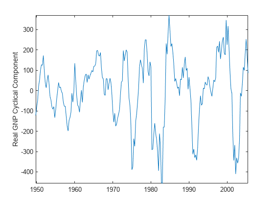
Plot the cyclical component of the US post-WWII, seasonally adjusted, quarterly, real gross national product (GNPR).
load Data_GNP
GNPR = Data(:,2);
[trend,cyclical] = hfilter(GNPR);
T = numel(trend)
T = 235
trend and cyclical are 235-by-1 vectors containing the trend and cyclical components, respectively, resulting from applying the Hamilton filter to the series with default lead and lag lengths. The first 7 values are NaNs.
plot(dates,cyclical)
axis tight
ylabel("Real GNP Cyclical Component")
Apply the Hamilton filter to all variables in input table variables.
Load the Schwert stock data set Data_SchwertStock.mat, which contains monthly returns of the NYSE index from 1871 through 2008 in DataTimeTableMth, among three other variables (for details, enter Description). Remove all missing observations from all series.
load Data_SchwertStock
TTM = rmmissing(DataTimeTableMth);
Aggregate the monthly data in the timetable to quarterly measurements.
TTQ = convert2quarterly(TTM);
Apply the Hamilton filter to all variables in the quarterly timetable. Use the default lead and lag lengths.
[TQTT,CQTT] = hfilter(TTQ);
size(TQTT)
ans = 1×2

   220     4
TQTT and CQTT are 220-by-4 timetables containing the trend and cyclical components, respectively, of the series in TTQ. Variables in the input and output timetables correspond. By default, hfilter filters all variables in the input table or timetable. To select a subset of variables, set the DataVariables option.
The default lead and lag lengths are 4. Consequently, the first 7 rows in the output timetable are NaN-valued.
Remove the leading and lagging NaNs from the trends and display what remains.
TQTTCut = rmmissing(TQTT);
CQTTCut = rmmissing(CQTT);
TQTTCut
TQTTCut=209×4 timetable
       Time          Return       DivYld        CapGain       CapGainA
    ___________    __________    _________    ___________    ___________

    31-Dec-1873     0.0052994    0.0037312    -0.00091529     0.00032353
    31-Mar-1874     0.0028083     0.003099     -0.0024575     -0.0018408
    30-Jun-1874     0.0028806    0.0041575     -0.0027131     -0.0019406
    30-Sep-1874     0.0033883    0.0030027     -0.0018109     -0.0014369
    31-Dec-1874     0.0053945    0.0032678     8.5274e-05     0.00027652
    31-Mar-1875     0.0051083    0.0026911      0.0007776     0.00072217
    30-Jun-1875     0.0035854    0.0032398    -0.00070225    -0.00041718
    30-Sep-1875     0.0081389    0.0037002      0.0032879      0.0045539
    31-Dec-1875     0.0052623    0.0029082     0.00081654     0.00098183
    31-Mar-1876     0.0074993    0.0033872      0.0030136      0.0029454
    30-Jun-1876    -0.0024581    0.0033423     -0.0052757     -0.0060788
    30-Sep-1876      0.006896    0.0022414    -0.00079166     0.00056363
    31-Dec-1876     0.0041519    0.0043172     0.00012738    -8.1701e-06
    31-Mar-1877     0.0035486    0.0025065     -0.0013859      -0.001144
    30-Jun-1877     0.0049609    0.0041852     0.00028714     0.00045375
    30-Sep-1877     0.0043711    0.0038399     0.00039172     0.00027915
      ⋮
CQTTCut
CQTTCut=209×4 timetable
       Time          Return        DivYld         CapGain       CapGainA
    ___________    __________    ___________    ___________    __________

    31-Dec-1873       0.12276     -0.0018286         0.0963       0.12583
    31-Mar-1874      -0.02564     -0.0010152      -0.010496     -0.023075
    30-Jun-1874    3.9596e-05     -0.0010583      -0.002827     0.0017616
    30-Sep-1874      0.016762     -0.0027748       0.018478      0.021359
    31-Dec-1874    -0.0067498       0.001779     -0.0028101    -0.0066786
    31-Mar-1875      0.012784     0.00012197       0.010181      0.014357
    30-Jun-1875     -0.011816     0.00066183       -0.02152     -0.011715
    30-Sep-1875     -0.020076    -4.8708e-05      -0.014556     -0.020143
    31-Dec-1875    -0.0097873    -0.00063718    -0.00081654    -0.0077777
    31-Mar-1876     -0.011327     -0.0013573     -0.0057609    -0.0088029
    30-Jun-1876     0.0094729      0.0010775    -0.00067668     0.0086738
    30-Sep-1876     -0.061711      0.0034416      -0.059335     -0.061062
    31-Dec-1876     0.0017068      0.0025794     -0.0070239    -0.0010298
    31-Mar-1877     -0.040981        0.00309      -0.050659     -0.041885
    30-Jun-1877      -0.09557      0.0024379      -0.072017     -0.097686
    30-Sep-1877      0.059143      0.0020562       0.060833      0.057339
      ⋮
To compare outputs between different tabular inputs, apply the Hamilton filter to all variables in the table of monthly data DataTableMth and the timetable of monthly data TTM.
% Table input of daily data
DTM = rmmissing(DataTableMth);
[TMDT,CMDT] = hfilter(DTM);
TMDT = rmmissing(TMDT);
CMDT = rmmissing(CMDT);
size(TMDT)
ans = 1×2
645 4
tail(TMDT)
                Return       DivYld       CapGain       CapGainA
               _________    _________    __________    __________

    May1925    0.0076851    0.0035499     0.0033316     0.0032399
    Jun1925     0.007946    0.0055856     0.0038195     0.0037338
    Jul1925     0.010239    0.0044464     0.0063502     0.0063067
    Aug1925    0.0080799    0.0035821      0.003389     0.0037078
    Sep1925    0.0076608    0.0055354     0.0037118      0.003575
    Oct1925    0.0081879     0.004496     0.0042474     0.0041497
    Nov1925     0.005312    0.0034493    0.00060642    0.00071388
    Dec1925     0.009001    0.0049537     0.0052133     0.0048893
tail(CMDT)
                 Return        DivYld        CapGain       CapGainA
               __________    ___________    __________    __________

    May1925      0.058501     -0.0010668      0.060371      0.060463
    Jun1925    -0.0047057    -0.00012725    -0.0060375    -0.0059518
    Jul1925     0.0086164     0.00076594     0.0072928     0.0073363
    Aug1925      0.040128    -0.00087019      0.042107      0.041788
    Sep1925     0.0091173    -0.00023334     0.0077642      0.007901
    Oct1925      0.060009     0.00014365       0.05931      0.059407
    Nov1925     -0.013777    -0.00063483     -0.011885     -0.011993
    Dec1925       0.04059      0.0021392      0.037285      0.037609
% Timetable input of daily data
[TMTT,CMTT] = hfilter(TTM);
TMTT = rmmissing(TMTT);
CMTT = rmmissing(CMTT);
size(TMTT)
ans = 1×2
645 4
tail(TMTT)
       Time         Return       DivYld       CapGain       CapGainA
    ___________    _________    _________    __________    __________

    01-May-1925    0.0076851    0.0035499     0.0033316     0.0032399
    01-Jun-1925     0.007946    0.0055856     0.0038195     0.0037338
    01-Jul-1925     0.010239    0.0044464     0.0063502     0.0063067
    01-Aug-1925    0.0080799    0.0035821      0.003389     0.0037078
    01-Sep-1925    0.0076608    0.0055354     0.0037118      0.003575
    01-Oct-1925    0.0081879     0.004496     0.0042474     0.0041497
    01-Nov-1925     0.005312    0.0034493    0.00060642    0.00071388
    01-Dec-1925     0.009001    0.0049537     0.0052133     0.0048893
tail(CMTT)
       Time          Return        DivYld        CapGain       CapGainA
    ___________    __________    ___________    __________    __________

    01-May-1925      0.058501     -0.0010668      0.060371      0.060463
    01-Jun-1925    -0.0047057    -0.00012725    -0.0060375    -0.0059518
    01-Jul-1925     0.0086164     0.00076594     0.0072928     0.0073363
    01-Aug-1925      0.040128    -0.00087019      0.042107      0.041788
    01-Sep-1925     0.0091173    -0.00023334     0.0077642      0.007901
    01-Oct-1925      0.060009     0.00014365       0.05931      0.059407
    01-Nov-1925     -0.013777    -0.00063483     -0.011885     -0.011993
    01-Dec-1925       0.04059      0.0021392      0.037285      0.037609
Because the data is disaggregated, the outputs of the daily data have more rows than from the quarterly data. The filter results of the daily inputs are equal among the corresponding outputs, but hfilter returns tables of results, instead of timetables, when you supply data in a table.
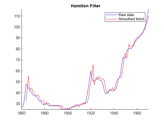
Load the Nelson-Plosser macroeconomic data set Data_NelsonPlosser.mat, which contains series measured yearly in the timetable DataTimeTable.
load Data_NelsonPlosserApply the Hamilton filter to the real and nominal GNP series, GNPR and GNPN, respectively. Set the lead and lag lengths 2 years and 1 year, respectively. Plot the trend component with each series.
hfilter(DataTimeTable,DataVariables=["GNPR" "GNPN"], ...
    LeadLength=2,LagLength=3);

Experiment with filter parameter values by adjusting the interactive controls.
varnames = string(DataTimeTable.Properties.VariableNames); lead =2; % LeadLength lag =
3; % LagLength vn =
varnames(8); % DataVariables figure [TTbl,CTbl,h] = hfilter(DataTimeTable,DataVariables=vn, ... LeadLength=lead,LagLength=lag);
Input Arguments
Name-Value Arguments
Output Arguments
More About
Tips
Regarding a setting for the
LeadLengthname-value argument, Hamilton [2] states "If we are interested in business cycles, a 2-year horizon should be the standard benchmark." Regarding a setting for theLagLengthname-value argument, the article states "One might be tempted to use a richer model to forecast yt+h, such as using more than 4 lags, or even a nonlinear relation. However, such refinements are completely unnecessary for the goal of extracting a stationary (cyclical) component, and have the significant drawback that the more parameters we try to estimate by regression, the more the small-sample results are likely to differ from the asymptotic predictions."
References
Version History
Introduced in R2023a