Analyze US Unemployment Rate Using Markov-Switching Model
This example shows how to fit a univariate Markov-switching dynamic regression model of the US unemployment rate to time series data. Also, the example shows how to simulate and forecast unemployment rate paths from the estimated model.
To fit a Markov-switching model for a univariate time series variable to data by using the estimate function, follow this general procedure:
Load and preprocess the time series data that you plan to model.
Examine the data to determine the key characteristics of the model, which include the number of states that the variable switches among and the structure of the state-specific submodels. Plots of the data or economic theory and principles can suggest the number of states. The structure of each submodel should be parsimonious and a good statistical description of the time series within the regime.
Create a partially specified Markov-switching model template for estimation by using the
msVARfunction. The model template, anmsVARobject, specifies the structure of each state submodel and the switching mechanism among the submodels, and the parameters to fit to data.Create a fully specified Markov-switching model that has the same structure as the model template. The
estimatefunction uses the parameter values of this model to initialize the estimation procedure, which is the expectation-maximization algorithm.Estimate the model by supplying
estimatewith the model template, initial model, and the data.
After fitting the model to data, you can pass the estimated model to the appropriate function for further analysis. For example, you can forecast the unemployment rate beyond the sample by using the forecast or simulate functions.
Load and Preprocess Data
Load the US unemployment data set in Data_Unemployment.mat. The data set contains the monthly rates from 1954 through 1998.
load Data_UnemploymentThe data set contains the 45-by-12 matrix Data and the numeric vector of observation years dates, among other variables (for more details, enter Description at the command line). Rows of Data correspond to the years 1954 through 1998 and columns correspond to the months January through December.
Econometrics Toolbox™ functions accept time series data with observations along the rows and separate variables along the columns of arrays. Reorient the rate series as one column vector containing all observations in increasing time order.
Data = Data';
un = Data(:);
un is a column vector containing the monthly unemployment rate series.
Create a datetime vector containing the observation times. Assume measurements are available at the beginning of each month.
numYears = numel(dates);
t = datetime(dates(1),1,1) + calmonths(0:((12*numYears)-1));
numObs = numel(t);
Examine Data
To determine key characteristics of the model, plot the entire unemployment rate series. Graphically distinguish periods of economic recession in the US, as determined by the National Bureau of Economic Research (NBER), by using the recessionplot function.
figure
plot(t,un)
recessionplot
ylabel("Rate (%)")
title("US Unemployment Rate, 1954-1998")
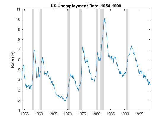
Gray bands indicate periods of recession. During each recession, the rate series increases sharply with visually similar statistical characteristics, such as strong autocorrelation (perhaps close to 0.9) and volatility, among those periods. Similarly, outside periods of recession, the rate decreases with similar statistical characteristics among those periods. However, the statistical characteristics of the series within recessions and expansion periods appear different. Therefore, the plot suggests that the unemployment rate might switch between two states or submodels, and each state-specific submodel likely has an autoregressive (AR) component.
Create Model Template for Estimation
An msVAR object is a variable that specifies a Markov-switching model; the msVAR function creates an msVAR object. For a univariate system, the function requires the following two inputs, which specify the key statistical characteristics of the model:
A vector of
arimaobjects, where element specifies the ARX() submodel in regime . Create each submodel by using thearimafunction. An analysis of the series within each regime, or economic theory, can suggest structures for the submodels, such as which AR lags to include. Note, however, complex model descriptions, such as those with many parameters, are a challenge for the optimization routine to fit to limited data and can result in high standard errors. A best practice is to specify parsimonious models that provide a good statistical description of the response series within the respective regimes. Also, simpler models tend to generalize better than complex models.A
dtmcobject, as created by thedtmcfunction, that represents the discrete-time Markov chain that describes the switching mechanism among the regimes.
Markov-switching model estimation requires the following two types of msVAR model objects:
A partially specified object that serves as a template explicitly specifying the model structure and indicating which parameters to estimate. Although you must specify all the non-estimable, structural parameters, such as lags in the AR polynomial, estimable parameters, such as lag coefficients and transition probabilities, can be unknown (
NaN-valued) or specified.estimatefitsNaN-valued parameters to the data and fixes all known parameters to their specified values.A fully specified object, with the same model structure as the template, that specifies the initial values of all parameters for the optimization algorithm.
To show how to use the msVAR framework, this example sets each submodel to an AR(1) model. However, you can base your choice on submodel structures by following this procedure:
Fit a set of models with varying, but not overly complex, submodel structures.
Choose the model that performs the best. Performance measures can include in-sample fit statistics, such as AIC, or forecast MSE from a holdout sample.
Specify the structure of each state submodel by creating a vector of AR(1) model templates.
statenames = ["Expansion" "Recession"];
mdl1 = arima(Constant=NaN,AR=NaN,Description=statenames(1));
mdl2 = arima(Constant=NaN,AR=NaN,Description=statenames(2));
submdl = [mdl1 mdl2];
mdl1
mdl1 =
  arima with properties:

     Description: "Expansion"
      SeriesName: "Y"
    Distribution: Name = "Gaussian"
               P: 1
               D: 0
               Q: 0
        Constant: NaN
              AR: {NaN} at lag [1]
             SAR: {}
              MA: {}
             SMA: {}
     Seasonality: 0
            Beta: [1×0]
        Variance: NaN

   ARIMA(1,0,0) Model (Gaussian Distribution)
mdl1 and mdl2 are partially specified arima objects representing AR(1) models containing a constant. The NaN-valued properties indicate which parameters to estimate. In this case and for state , the parameters are the constant , first AR lag , and innovation variance .
Create a two-state discrete-time Markov chain. Specify an unknown transition matrix.
mc = dtmc([NaN NaN; NaN NaN],StateNames=statenames)
mc =
  dtmc with properties:

             P: [2x2 double]
    StateNames: ["Expansion"    "Recession"]
     NumStates: 2
mc is a partially specified dtmc object representing the switching mechanism. Because the transition matrix is composed of NaN values, it is prepared for estimation.
Create a Markov-switching model template for estimation by supplying the partially specified submodel vector and switching mechanism to msVAR. Specify the state names.
Mdl = msVAR(mc,submdl)
Mdl =
  msVAR with properties:

      NumStates: 2
      NumSeries: 1
     StateNames: ["Expansion"    "Recession"]
    SeriesNames: "1"
         Switch: [1x1 dtmc]
      Submodels: [2x1 varm]
Mdl is a partially specified msVAR object specifying the Markov-switching model structure for estimation. Ten parameters are unknown, or correspond to NaN-valued properties, so estimate estimates them.
Create Model Containing Initial Values
The estimate function uses the expectation-maximization (EM) algorithm to optimize the data likelihood. The EM algorithm requires initial parameter values. estimate uses the parameter values of an input, fully specified Markov-switching model as the required initial values. Specified initial values do not need to be evidence based, but it is good practice to experiment with several sets of initial values to determine whether the algorithm is sensitive to them.
Base the starting values on visual inspection of the plot:
Because the plot suggests high positive autocorrelation in both states, set the initial first AR lag to 0.9.
Choose levels (unconditional means) of the rate as 4, for expansion, and 8, for recession.
Obtain the initial value for the constants by using these choices and the formula for the unconditional mean of a stationary AR(1) model, which is .
phi0 = 0.9;
muexp = 4;
murec = 8;
c0exp = muexp*(1 - phi0);
c0rec = murec*(1 - phi0);
Create a Markov-switching model of containing initial values for estimation. Arbitrarily set each state submodel variance to 1 and specify that transitions between states are uniformly distributed.
sigma20= 1;
mdl10 = arima(Constant=c0exp,AR=phi0,Variance=sigma20);
mdl20 = arima(Constant=c0rec,AR=phi0,Variance=sigma20);

P0 = 0.5*ones(2);
mc0 = dtmc(P0,StateNames=statenames);

Mdl0 = msVAR(mc0,[mdl10 mdl20]);
Mdl0 is a fully specified msVAR object containing the initial values for estimation.
Estimate Model
Fit the Markov-switching model to the entire unemployment rate series. Monitor convergence of the algorithm by plotting the log-likelihood for each iteration.
EstMdl = estimate(Mdl,Mdl0,un,IterationPlot=true);
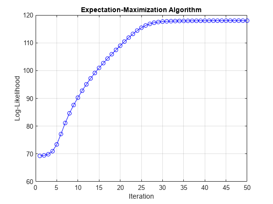
The monotonically increasing log-likelihood is indicative of the behavior of the EM algorithm. The algorithm terminates after about 50 iterations, when a consecutive change is below the tolerance, as specified by the Tolerance name-value argument.
EstMdl is a fully specified msVAR object representing the estimated Markov-switching model. The submodels are of the same structure as those in the model template, but all parameter values are specified.
Display an estimation summary.
summarize(EstMdl)
Description
1-Dimensional msVAR Model with 2 Submodels

Switch
Estimated Transition Matrix:
0.978 0.022
0.065 0.935

Fit
Effective Sample Size: 539
Number of Estimated Parameters: 4
Number of Constrained Parameters: 0
LogLikelihood: 117.978
AIC: -227.955
BIC: -210.796

Submodels
                           Estimate    StandardError    TStatistic      PValue
                           ________    _____________    __________    __________

    State 1 Constant(1)    0.09672        0.021617        4.4744      7.6639e-06
    State 1 AR{1}(1,1)     0.97007       0.0044692        217.06               0
    State 2 Constant(1)    0.10835        0.046026         2.354        0.018572
    State 2 AR{1}(1,1)     0.99926       0.0079809        125.21               0
A standard statistical summary prints to the command window, including parameter estimates and their standard errors and inferences, and model fit statistics.
Plot the estimated switching mechanism.
figure
graphplot(EstMdl.Switch,ColorEdges=true,LabelEdges=true)
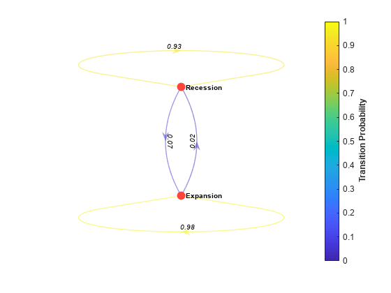
The estimated transition matrix Switch suggests that the states are sticky, meaning they have a high probability of persisting into the next time step. This characteristic is apparent in the time series plot.
The estimated Markov-switching model is
All estimates are significant at 5% level of significance.
Plot the estimated switching mechanism,.
Forecast Unemployment Rate
A fully specified msVAR object represents a known Markov-switching model, which you can pass to several functions for further analysis. For example, the msVAR framework supports both optimal and Monte-Carlo-based point forecasting from the forecast function. You can also generate random response paths from a model by using the simulate function.
Forecast Using forecast
Forecast the estimated model 120 months beyond the in-sample measurements. Compute optimal point forecasts.
numPeriods = 120;
unOPF = forecast(EstMdl,un,numPeriods);
unOPF is a 120-by-1 vector, in which unOPF(j) is the j-period-ahead optimal point forecast of the unemployment rate.
Compute Monte-Carlo-based forecasts by calling forecast again and returning the Monte-Carlo-based forecast variance (the second output argument). Base the forecasts on 1000 simulated paths.
rng(1) % For reproducibility
numPaths = 1000;
[unMCF,estVar] = forecast(EstMdl,un,numPeriods, ...
    NumPaths=numPaths);
unMCF and estVar are 120-by-1 vectors, where unMCF(j) and estVar(j) are the mean and variance, respectively, of the simulated unemployment rate paths at period j.
Plot the observed series with the optimal and Monte Carlo forecasts. Compute and plot point-wise 95% Wald confidence intervals for the forecasts.
hrzn = t(end) + calmonths(1:numPeriods);
MCFCI1 = unMCF + 1.96*[-estVar estVar];

figure
hold on
h1 = plot(t((end-300):end),un((end-300):end),"b");
h2 = plot(hrzn,unOPF,"r");
h3 = plot(hrzn,unMCF,"m");
h4 = plot(hrzn,MCFCI1,"--m");
hold off
title("Forecast Unemployment Rate")
legend([h1 h2 h3 h4(1)], ...
    ["Observed" "Optimal forecast" "MC forecast" "95% confidence interval"], ...
    Location="best")
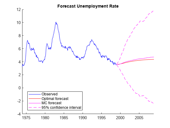
The plot suggests that the uncertainty on the unemployment rate far from the in-sample data is high. In fact, the intervals are wide enough to include impossible values of an unemployment rate.
Forecast Using simulate
To customize a Monte Carlo study, use simulate to generate random response paths from a model.
To see how Markov-switching model simulation works, simulate one path from the estimated model, and then plot the path with the data.
rng(1)
unsim = simulate(EstMdl,numObs);

figure
plot(t,un,'b',t,unsim,'r')
legend("Observed","Simulated")
title("Simulated Unemployment Rate")
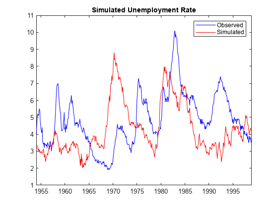
unsim is a numObs-by-1 vector containing a random path simulated from EstMdl. The simulated path shows short clusters of sharp increases and longer clusters of slower decreases, as demonstrated by the observed series.
Forecast the estimated Markov-switching model beyond the in-sample measurements by simulating 1000 paths, computing the time-point-wise simulation means and 95% percentile intervals. Supply the in-sample data as a presample. Plot the data, the first simulated path, and the Monte Carlo forecasts and inferences.
UNMCSim = simulate(EstMdl,numPeriods,NumPaths=numPaths,Y0=un);

unmcmean = mean(UNMCSim,2);
unmcint = quantile(UNMCSim,[0.025 0.975],2);

figure
h1 = plot(t(end-300:end),un(end-300:end),"k");
hold on
h2 = plot(hrzn,UNMCSim(:,1),"r");
h3 = plot(hrzn,unmcmean,"m");
h4 = plot(hrzn,unmcint,"--m");
h5 =gca;
patch([hrzn(1) h5.XLim(2) h5.XLim(2) hrzn(1)],[h5.YLim([1 1]) h5.YLim([2 2])], ...
    [0.75 0.75 0.75],FaceAlpha=0.2)
hold off
legend([h1 h2 h3 h4(1)], ...
    ["Observed" "Simulated path" "MC forecast" "95% confidence intervals"], ...
    Location="best")
title("Monte Carlo Forecasted Unemployment Rate")

UNMCSim is a 120-by-1000 matrix, where rows correspond to periods in the forecast horizon and columns are separate, independently simulated response paths.
Like the Wald-based confidence intervals, the percentile intervals of forecasts far from the in-sample data are wide, but the values contained in them are possible.
See Also
Objects
Functions
Related Topics
Select a Web Site
Choose a web site to get translated content where available and see local events and offers. Based on your location, we recommend that you select: United States.
You can also select a web site from the following list
Americas
- América Latina (Español)
- Canada (English)
- United States (English)
Europe
- Belgium (English)
- Denmark (English)
- Deutschland (Deutsch)
- España (Español)
- Finland (English)
- France (Français)
- Ireland (English)
- Italia (Italiano)
- Luxembourg (English)
- Netherlands (English)
- Norway (English)
- Österreich (Deutsch)
- Portugal (English)
- Sweden (English)
- Switzerland
- United Kingdom (English)
Asia Pacific
- Australia (English)
- India (English)
- New Zealand (English)
- 中国
- 日本Japanese (日本語)
- 한국Korean (한국어)