simulate
Simulate sample paths of Markov-switching dynamic regression model
Description
Y = simulate(Mdl,numObs,Name,Value)'NumPaths',1000,'Y0',Y0 simulates 1000 sample paths and initializes the dynamic component of each submodel by using the presample response data Y0.
[ also returns the simulated innovation paths Y,E,StatePaths] = simulate(___)E and the simulated state paths StatePaths, using any of the input argument combinations in the previous syntaxes.
Examples
Simulate a response path from a two-state Markov-switching dynamic regression model for a 1-D response process. This example uses arbitrary parameter values.
Create Fully Specified Model
Create a two-state discrete-time Markov chain model that describes the regime switching mechanism. Label the regimes.
P = [0.9 0.1; 0.3 0.7];
mc = dtmc(P,'StateNames',["Expansion" "Recession"]);
mc is a fully specified dtmc object.
For each regime, use arima to create an AR model that describes the response process within the regime. Store the submodels in a vector.
mdl1 = arima('Constant',5,'AR',[0.3 0.2],...
    'Variance',2);
mdl2 = arima('Constant',-5,'AR',0.1,...
    'Variance',1);
mdl = [mdl1; mdl2];
mdl1 and mdl2 are fully specified arima objects.
Create a Markov-switching dynamic regression model from the switching mechanism mc and the vector of submodels mdl.
Mdl = msVAR(mc,mdl);
Mdl is a fully specified msVAR object.
Simulate Response Path
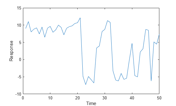
Generate one random response path of length 50 from the model.
rng(1); % For reproducibility
y = simulate(Mdl,50);
y is a 50-by-1 vector of one response path.
Plot the response path.
figure
plot(y)
xlabel("Time")
ylabel("Response")
Consider the model in Simulate Response Path.
Create the Markov-switching dynamic regression model.
P = [0.9 0.1; 0.3 0.7];
mc = dtmc(P,'StateNames',["Expansion" "Recession"]);
mdl1 = arima('Constant',5,'AR',[0.3 0.2],...
    'Variance',2);
mdl2 = arima('Constant',-5,'AR',0.1,...
    'Variance',1);
mdl = [mdl1; mdl2];
Mdl = msVAR(mc,mdl);
Simulate 3 response, innovations, and state-index paths of 5 observations from the model.
rng('default') % For reproducibility
[Y,E,SP] = simulate(Mdl,5,'NumPaths',3)
Y = 5×3

   -5.7605   10.9496   11.4633
   -5.7002    8.5772   -3.1268
    4.2446   10.7774   -5.6161
   -3.1665   -2.2920   -5.2677
   -3.8995   -4.7403   -6.3141
E = 5×3

   -0.2050    0.9496    1.4633
   -0.1241   -1.7076    0.7269
    2.1068    1.0143   -0.3034
    1.4090    1.6302    0.2939
    1.4172    0.4889   -0.7873
SP = 5×3

     2     1     1
     2     1     2
     1     1     2
     2     2     2
     2     2     2
Y, E, and SP are 5-by-3 matrices. Columns represent separate, independent paths.
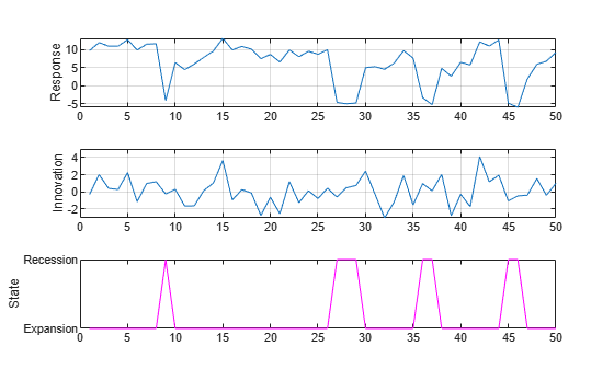
Simulate a single path of responses, innovations, and states into a simulation horizon of length 50. Then plot each path separately.
[y,e,sp] = simulate(Mdl,50);

figure
subplot(3,1,1)
plot(y)
ylabel('Response')
grid on
subplot(3,1,2)
plot(e)
ylabel('Innovation')
grid on
subplot(3,1,3)
plot(sp,'m')
ylabel('State')
yticks([1 2])
yticklabels(Mdl.StateNames)
Consider a two-state Markov-switching dynamic regression model of the postwar US real GDP growth rate. The model has the parameter estimates presented in [1].
Create a discrete-time Markov chain model that describes the regime switching mechanism. Label the regimes.
P = [0.92 0.08; 0.26 0.74];
mc = dtmc(P,'StateNames',["Expansion" "Recession"]);
Create separate AR(0) models (constant only) for the two regimes.
sigma = 3.34; % Homoscedastic models across states
mdl1 = arima('Constant',4.62,'Variance',sigma^2);
mdl2 = arima('Constant',-0.48,'Variance',sigma^2);
mdl = [mdl1 mdl2];
Create the Markov-switching dynamic regression model that describes the behavior of the US GDP growth rate.
Mdl = msVAR(mc,mdl);
Mdl is a fully specified msVAR object.
Generate one random path of 100 responses, corresponding innovations, and states from the model.
rng(1) % For reproducibility
[y,e,sp] = simulate(Mdl,100);
y is a 100-by-1 vector of GDP rates, and e is a 100-by-1 vector of corresponding innovations. sp is a 100-by-1 vector of state indices.
Consider the Markov-switching model in Simulate US GDP Rates and Economic States, but assume that the submodels are AR(1) instead. Consider fitting the model to observations in the period 1960:Q1–2004:Q2.
Create the model template for estimation. Specify AR(1) submodels.
mc = dtmc(NaN(2),'StateNames',["Expansion" "Recession"]);
ar1 = arima(1,0,0);
Mdl = msVAR(mc,[ar1; ar1]);
Because the submodels are AR(1), each requires one presample observation to initialize its dynamic component for estimation.
Create the model containing initial parameter values for the estimation procedure.
mc0 = dtmc(0.5*ones(2),'StateNames',["Expansion" "Recession"]);
submdl01 = arima('Constant',1,'Variance',1,'AR',0.001);
submdl02 = arima('Constant',-1,'Variance',1,'AR',0.001);
Mdl0 = msVAR(mc0,[submdl01; submdl02]);
Load the data. Transform the entire set to an annualized rate series.
load Data_GDP
qrate = diff(Data)./Data(1:(end - 1));
arate = 100*((1 + qrate).^4 - 1);
Identify the presample and estimation sample periods using the dates associated with the annualized rate series. Because the transformation applies the first difference, you must drop the first observation date from the original sample.
dates = datetime(dates(2:end),'ConvertFrom','datenum',...
    'Format','yyyy:QQQ','Locale','en_US');
estPrd = datetime(["1960:Q2" "2004:Q2"],'InputFormat','yyyy:QQQ',...
    'Format','yyyy:QQQ','Locale','en_US');
idxEst = isbetween(dates,estPrd(1),estPrd(2));
idxPre = dates < estPrd(1);
Fit the model to the estimation sample data. Specify the presample observation.
y0 = arate(idxPre);
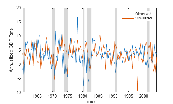
EstMdl = estimate(Mdl,Mdl0,arate(idxEst),'Y0',y0);Simulate a response path from the fitted model over the estimation period. Specify the presample observation.
rng(1) % For reproducibility
numObs = sum(idxEst);
aratesim = simulate(EstMdl,numObs,'Y0',y0);
Plot the observations and simulated path of annualized rates, and identify periods of recession by using recessionplot.
figure;
plot(dates(idxEst),[arate(idxEst) aratesim])
recessionplot
xlabel("Time")
ylabel("Annualized GDP Rate")
legend("Observed","Simulated");
Assess estimation accuracy using simulated data from a known data-generating process (DGP). This example uses arbitrary parameter values.
Create Model for DGP
Create a fully specified, two-state discrete-time Markov chain model for the switching mechanism.
P = [0.7 0.3; 0.1 0.9];
mc = dtmc(P);
For each state, create a fully specified AR(1) model for the response process.
% Constants
C1 = 5;
C2 = -2;

% Autoregression coefficients
AR1 = 0.4;
AR2 = 0.2;

% Variances
V1 = 4;
V2 = 2;

% AR Submodels
dgp1 = arima('Constant',C1,'AR',AR1,'Variance',V1);
dgp2 = arima('Constant',C2,'AR',AR2,'Variance',V2);
Create a fully specified Markov-switching dynamic regression model for the DGP.
DGP = msVAR(mc,[dgp1,dgp2]);
Simulate Response Paths from DGP
Generate 10 random response paths of length 1000 from the DGP.
rng(1); % For reproducibility
N = 10;
n = 1000;
Data = simulate(DGP,n,'Numpaths',N);
Data is a 1000-by-10 matrix of simulated responses.
Create Model for Estimation
Create a partially specified Markov-switching dynamic regression model that has the same structure as the data-generating process, but specify an unknown transition matrix and unknown submodel coefficients.
PEst = NaN(2);
mcEst = dtmc(PEst);
mdl = arima(1,0,0);
Mdl = msVAR(mcEst,[mdl; mdl]);
Create Model Containing Initial Values
Create a fully specified Markov-switching dynamic regression model that has the same structure as Mdl, but set all estimable parameters to initial values.
P0 = 0.5*ones(2);
mc0 = dtmc(P0);
mdl01 = arima('Constant',1,'AR',0.5,'Variance',2);
mdl02 = arima('Constant',-1,'AR',0.5,'Variance',1);
Mdl0 = msVAR(mc0,[mdl01,mdl02]);
Estimate Models
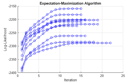
Fit the model to each simulated path. For each path, plot the loglikelihood at each iteration of the EM algorithm.
c1 = zeros(N,1);
c2 = zeros(N,1);
v1 = zeros(N,1);
v2 = zeros(N,1);
ar1 = zeros(N,1);
ar2 = zeros(N,1);
PStack = zeros(2,2,N);

figure
hold on

for i = 1:N

    EstModel = estimate(Mdl,Mdl0,Data(:,i),'IterationPlot',true);

    c1(i) = EstModel.Submodels(1).Constant;
    c2(i) = EstModel.Submodels(2).Constant;
    v1(i) = EstModel.Submodels(1).Covariance;
    v2(i) = EstModel.Submodels(2).Covariance;
    ar1(i) = EstModel.Submodels(1).AR{1};
    ar2(i) = EstModel.Submodels(2).AR{1};
    PStack(:,:,i) = EstModel.Switch.P;

end

hold off
Assess Accuracy
Compute the Monte Carlo mean of each estimated parameter.
c1Mean = mean(c1);
c2Mean = mean(c2);
v1Mean = mean(v1);
v2Mean = mean(v2);
ar1Mean = mean(ar1);
ar2Mean = mean(ar2);
PMean = mean(PStack,3);
Compare population parameters to the corresponding Monte Carlo estimates.
DGPvsEstimate = [...
    C1  c1Mean
    C2  c2Mean
    V1  v1Mean
    V2  v2Mean
    AR1 ar1Mean
    AR2 ar2Mean]
DGPvsEstimate = 6×2
5.0000 5.0260
-2.0000 -1.9615
4.0000 3.9710
2.0000 1.9903
0.4000 0.4061
0.2000 0.2017
P
P = 2×2

    0.7000    0.3000
    0.1000    0.9000
PEstimate = PMean
PEstimate = 2×2

    0.7065    0.2935
    0.1023    0.8977
Generate random paths from a three-state Markov-switching dynamic regression model for a 2-D VARX response process. This example uses arbitrary parameter values for the DGP.
Create Fully Specified Model for DGP
Create a three-state discrete-time Markov chain model for the switching mechanism.
P = [10 1 1; 1 10 1; 1 1 10];
mc = dtmc(P);
mc is a fully specified dtmc object. dtmc normalizes the rows of P so that they sum to 1.
For each regime, use varm to create a VAR model that describes the response process within the regime. Specify all parameter values.
% Constants
C1 = [1;-1];
C2 = [2;-2];
C3 = [3;-3];

% Autoregression coefficients
AR1 = {};
AR2 = {[0.5 0.1; 0.5 0.5]};
AR3 = {[0.25 0; 0 0] [0 0; 0.25 0]};

% Regression coefficients
Beta1 = [1;-1];
Beta2 = [2 2;-2 -2];
Beta3 = [3 3 3;-3 -3 -3];

% Innovations covariances
Sigma1 = [1 -0.1; -0.1 1];
Sigma2 = [2 -0.2; -0.2 2];
Sigma3 = [3 -0.3; -0.3 3];

% VARX submodels
mdl1 = varm('Constant',C1,'AR',AR1,'Beta',Beta1,'Covariance',Sigma1);
mdl2 = varm('Constant',C2,'AR',AR2,'Beta',Beta2,'Covariance',Sigma2);
mdl3 = varm('Constant',C3,'AR',AR3,'Beta',Beta3,'Covariance',Sigma3);
mdl = [mdl1; mdl2; mdl3];
mdl contains three fully specified varm model objects.
For the DGP, create a fully specified Markov-switching dynamic regression model from the switching mechanism mc and the submodels mdl.
Mdl = msVAR(mc,mdl);
Mdl is a fully specified msVAR model.
Simulate Data Ignoring Regression Component
If you do not supply exogenous data, simulate ignores the regression components in the submodels. Simulate 3 separate, independent paths of responses, innovations, and state indices of length 5 from the model.
rng(1); % For reproducibility
[Y,E,SP] = simulate(Mdl,5,'NumPaths',3)
Y =
Y(:,:,1) =

    5.2387    1.5297
    4.4290    4.2738
    1.1668   -1.2905
   -0.9654   -0.2028
   -0.2701    0.8993


Y(:,:,2) =

    2.7737   -2.5383
   -0.8651   -1.1046
   -0.0511    0.3696
    0.5826   -0.8926
    2.4022   -0.6912


Y(:,:,3) =

    3.5443    0.8768
    4.9748   -0.7956
    5.7213    0.8073
    4.2473    0.5805
    2.7972   -1.3340
E =
E(:,:,1) =

    1.2387    1.5297
   -0.3434    2.8896
    0.1668   -0.2905
   -1.9654    0.7972
   -1.2701    1.8993


E(:,:,2) =

    1.7737   -1.5383
   -1.8651   -0.1046
   -1.0511    1.3696
   -0.4174    0.1074
    1.4022    0.3088


E(:,:,3) =

   -0.4557    0.8768
    1.1150   -1.0061
    1.3134    0.7176
   -0.6941   -0.6838
    1.7972   -0.3340
SP = 5×3

     2     1     2
     2     1     2
     1     1     2
     1     1     2
     1     1     1
Y and E are 5-by-2-by-3 arrays of simulated responses and innovations, respectively. Rows correspond to time points, columns correspond to variables in the system, and pages correspond to paths. SP is a 5-by-3 matrix whose columns correspond to paths.
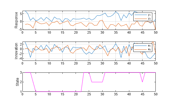
Simulate a single path of responses, innovations, and states into a simulation horizon of length 50. Then plot each path separately.
rng0 = rng; % Store settings to reproduce state sequence.
[Y,E,SP] = simulate(Mdl,50);

figure
subplot(3,1,1)
plot(Y)
ylabel("Response")
grid on
legend(["y_1" "y_2"])
subplot(3,1,2)
plot(E)
ylabel("Innovation")
grid on
legend(["e_1" "e_2"])
subplot(3,1,3)
plot(SP,'m')
ylabel("State")
yticks([1 2 3])
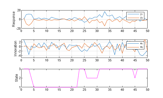
Simulate Data Including Regression Component
Simulate exogenous data for the three regressors by generating 50 random observations from the 3-D standard Gaussian distribution.
X = randn(50,3);
Generate one random response, innovation, and state path of length 50. Specify the simulated exogenous data for the submodel regression components. Plot the results.
rng(rng0); % Reproduce state sequence in previous simulation.
[Y,E,SP] = simulate(Mdl,50,'X',X);

figure
subplot(3,1,1)
plot(Y)
ylabel("Response")
grid on
legend(["y_1" "y_2"])
subplot(3,1,2)
plot(E)
ylabel("Innovation")
grid on
legend(["e_1" "e_2"])
subplot(3,1,3)
plot(SP,'m')
ylabel("State")
yticks([1 2 3])
Consider the model in Simulate Paths from Model with VARX Submodels.
Create Fully Specified Model
Create the Markov-switching model excluding the regression component.
P = [10 1 1; 1 10 1; 1 1 10];
mc = dtmc(P);
C1 = [1;-1];
C2 = [2;-2];
C3 = [3;-3];
AR1 = {};
AR2 = {[0.5 0.1; 0.5 0.5]};
AR3 = {[0.25 0; 0 0] [0 0; 0.25 0]};
Sigma1 = [1 -0.1; -0.1 1];
Sigma2 = [2 -0.2; -0.2 2];
Sigma3 = [3 -0.3; -0.3 3];
mdl1 = varm('Constant',C1,'AR',AR1,'Covariance',Sigma1);
mdl2 = varm('Constant',C2,'AR',AR2,'Covariance',Sigma2);
mdl3 = varm('Constant',C3,'AR',AR3,'Covariance',Sigma3);
mdl = [mdl1; mdl2; mdl3];
Mdl = msVAR(mc,mdl);
Simulate Multiple Paths
Generate 1000 random paths of responses for 50 time steps. Start all simulations at the first state.
rng(10); % For reproducibility
S0 = [1 0 0];
Y = simulate(Mdl,50,'S0',S0,'NumPaths',1000);
Y is a 50-by-2-by-1000 array of simulated response paths.
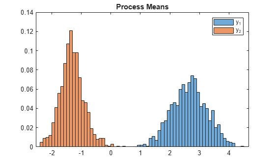
Compute Monte Carlo Distribution
For each variable and path, compute the process mean.
mus = mean(Y,1);
For each variable, plot the Monte Carlo distribution of the process mean.
figure
h1 = histogram(mus(1,1,:),'Normalization',"probability",...
    'BinWidth',0.1);
hold on
h2 = histogram(mus(1,2,:),'Normalization',"probability",...
    'BinWidth',0.1);
legend(["y_1" "y_2"])
title('Process Means')
hold off
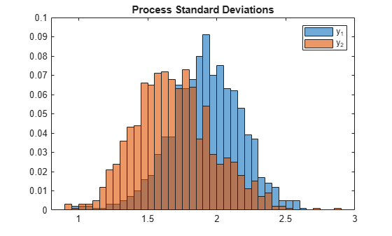
For each variable and path, compute the process standard deviation.
sigmas = std(Y,0,1);
For each variable, plot the Monte Carlo distribution of the process standard deviation.
figure
h1 = histogram(sigmas(1,1,:),'Normalization',"probability",...
    'BinWidth',0.05);
hold on
h2 = histogram(sigmas(1,2,:),'Normalization',"probability",...
    'BinWidth',0.05);
legend(["y_1" "y_2"])
title('Process Standard Deviations')
hold off
Input Arguments
Name-Value Arguments
Output Arguments
References
[1] Chauvet, M., and J. D. Hamilton. "Dating Business Cycle Turning Points." In Nonlinear Analysis of Business Cycles (Contributions to Economic Analysis, Volume 276). (C. Milas, P. Rothman, and D. van Dijk, eds.). Amsterdam: Emerald Group Publishing Limited, 2006.
[2] Hamilton, J. D. "Analysis of Time Series Subject to Changes in Regime." Journal of Econometrics. Vol. 45, 1990, pp. 39–70.
[3] Hamilton, James D. Time Series Analysis. Princeton, NJ: Princeton University Press, 1994.
Version History
Introduced in R2019b