Simulate Univariate Markov-Switching Dynamic Regression Model
This example shows how to generate random response and state paths from a two-state Markov-switching dynamic regression model.
Suppose that an economy switches between two regimes: an expansion and a recession. If the economy is in an expansion, the probability that the expansion persists in the next time step is 0.9, and the probability that it switches to a recession is 0.1. If the economy is in a recession, the probability that the recession persists in the next time step is 0.7, and the probability that it switches to a recession is 0.3.
Also suppose that is a univariate response process representing an economic measurement that can suggest which state the economy experiences during a period. During an expansion, is this AR(2) model:
where is an iid Gaussian process with mean 0 and variance 2. During a recession, is this AR(1) model:
where is an iid Gaussian process with mean 0 and variance 1.
Create Fully Specified Model
Create the Markov-switching dynamic regression model that describes the state of the economy with respect to .
% Switching mechanism
P = [0.9 0.1; 0.3 0.7];
mc = dtmc(P,StateNames=["Expansion" "Recession"]);

% AR submodels
mdl1 = arima(Constant=5,AR=[0.3 0.2],Variance=2, ...
    Description="Expansion State");
mdl2 = arima(Constant=-5,AR=0.1,Variance=1, ...
    Description="Recession State");

% Markov-switching model
Mdl = msVAR(mc,[mdl1; mdl2]);
Mdl is a fully specified msVAR object.
Simulate One Path
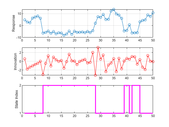
Simulate one path of responses, innovations, and state indices from the model. Specify a 50-period simulation horizon, that is, a 50-observation path.
rng("default")
[y,e,sp] = simulate(Mdl,50);y, e, and sp are 50-by-1 vectors of simulated responses, innovations, and state indices, respectively.
Plot the simulated observations in separate subplots.
figure
tiledlayout(3,1)
nexttile
plot(y,"o-")
ylabel("Response")
grid on

nexttile
plot(e,"ro-")
ylabel("Innovation")
grid on

nexttile
stairs(sp,"m",LineWidth=2)
ylabel("State Index")
yticks([1 2])
Simulate Multiple Paths
Simulate three separate, independent paths of responses, innovations, and state indices from the model. Specify a 5-period simulation horizon.
[Y,E,SP] = simulate(Mdl,5,NumPaths=3)
Y = 5×3

   -5.4315   14.1125    9.6147
   -4.1065   12.4008   11.4378
   -7.3715   13.4929   -4.1341
    1.6877   10.0315    7.0395
    2.3238   10.0453    3.3833
E = 5×3

    0.1240    4.1125   -0.3853
    1.4367    1.1670    1.5534
   -1.9609    1.9502   -0.2779
   -0.2796   -1.4965    0.9921
   -1.7082   -0.6627   -2.9017
SP = 5×3

     2     1     1
     2     1     1
     2     1     2
     1     1     1
     1     1     1
Mdl.StateNames(SP(2,1))
ans =
"Recession"
Y, E, and SP are 5-by-3 matrices of simulated responses, innovations, and state indices, respectively.
The simulated response in the second period of the first path is –4.1065.
The corresponding simulated innovation in the second period of the first path is 1.4367.
The corresponding simulated state of the economy in the second period of the first path is a recession.
Simulate Model Containing Regression Component
Include a known regression component in each submodel. During an expansion, the ARX(2) submodel is:
During a recession, the ARX(1) submodel is:
Specify the regression coefficient values of each submodel by setting the Beta property using dot notation. Then, create a new Markov-switching model from the modified ARX submodels and the existing Markov chain mc.
mdl1.Beta = 2;
mdl2.Beta = 1;
Mdl = msVAR(mc,[mdl1; mdl2]);
simulate requires exogenous data over the simulation horizon for the regression component. Generate a 50-by-1 matrix of iid standard normal observations for the required exogenous data.
x = randn(50,1);
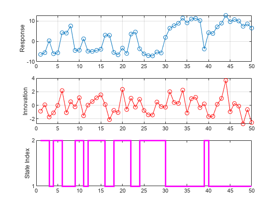
Simulate one path of responses, innovations, and state indices from the model. Specify a 50-period simulation horizon. Plot the results.
[y,e,sp] = simulate(Mdl,50,X=x);

figure
tiledlayout(3,1)
nexttile
plot(y,"o-")
ylabel("Response")
grid on

nexttile
plot(e,"ro-")
ylabel("Innovation")
grid on

nexttile
stairs(sp,"m",LineWidth=2)
ylabel("State Index")
yticks([1 2])