filterAnalyzer

Analyze filters with Filter Analyzer app

Since R2024a

Description

The filterAnalyzer object analyzes the responses of input filters using the Filter Analyzer app.

Creation

Syntax

filterAnalyzer

filterAnalyzer(filt1,...,filtn)

filterAnalyzer(filt1,...,filtn,Name=Value)

filterAnalyzer(filename)

filterAnalyzer(filename,"append")

[fa,dispnums] = filterAnalyzer(___)

Description

filterAnalyzer opens the Filter Analyzer app.

filterAnalyzer(filt1,...,filtn) plots the responses of the specified filters in the Filter Analyzer app.

• If Filter Analyzer is not open, this syntax opens the app and plots the responses.

• If Filter Analyzer is open, this syntax plots the responses in a new display in the app.

filterAnalyzer(filt1,...,filtn,Name=Value) specifies additional options using one or more name-value arguments. For example, you can specify filter names, sample rates, or analysis options.

filterAnalyzer(filename) opens a Filter Analyzer session stored in the specified MAT file filename. If Filter Analyzer is already open, this syntax replaces the current app session with the new session.

filterAnalyzer(filename,"append") appends the filters stored in the specified MAT file filename to the current Filter Analyzer session. If Filter Analyzer is not open, this syntax is equivalent to the previous syntax.

[fa,dispnums] = filterAnalyzer(___) returns a handle object for the Filter Analyzer and the numbers corresponding to the newly added displays, using any combination of input arguments from previous syntaxes.

You can also obtain the handle fa by typing fa = getFilterAnalyzerHandle at the command line.

Input Arguments

filt — Input filters

pair of coefficient matrices | cell array | digitalFilter object | filter System object™

Input filter, specified as one of these:

• A pair of coefficient matrices — Specify filt as two arguments B,A, where B and A are the numerator and denominator coefficients, respectively. For more information, see Import Filter Coefficients.

• A cell array — Specify filt as a cell array with the form {B,A,g}, where B and A are the numerator and denominator coefficients, respectively, and g represents the scaling gain of the filter. For more information, see Import Filter Coefficients.

• A digitalFilter object — Specify filt as a digitalFilter object. To generate or edit digital filters based on frequency-response specifications at the command line, use designfilt.

• A filter System object— Specify filt as a System object. For more information, see Supported Filter System Objects.

Example: B = [1 3 3 1]/6 and A = [3 0 1 0]/3 together specify a third-order lowpass Butterworth filter with a normalized 3 dB frequency of 0.5π rad/sample.

Example: [B,A] = sos2ctf([2 4 2 6 0 2; 3 3 0 6 0 0]) and g = [1;1;1] specify a third-order lowpass Butterworth filter with a normalized 3 dB frequency of 0.5π rad/sample and with scaling gains.

Example: d = designfilt("lowpassiir",FilterOrder=3,HalfPowerFrequency=0.5) specifies a third-order lowpass Butterworth filter with a normalized 3 dB frequency of 0.5π rad/sample.

Example: hd = design(fdesign.lowpass,"butter",SystemObject=true) specifies a lowpass Butterworth filter System object.

Data Types: single | double | int8 | int16 | int32 | int64 | uint8 | uint16 | uint32 | uint64 | cell
Complex Number Support: Yes

filename — Session filename

character vector | string scalar

Session filename, specified as a character vector or string scalar.

Example: 'lowpassdesigns.mat'

Example: "C:\MyFolder\myfilters.mat"

Data Types: char | string

Name-Value Arguments

Specify optional pairs of arguments as Name1=Value1,...,NameN=ValueN, where Name is the argument name and Value is the corresponding value. Name-value arguments must appear after other arguments, but the order of the pairs does not matter.

Example: filterAnalyzer(Analysis="impulse",OverlayAnalysis="step") specifies a step response analysis overlaid on an impulse response analysis.

Analysis — Analysis type

"magnitude" (default) | "phase" | "groupdelay" | "phasedelay" | "magestimate" | "noisepsd" | "impulse" | "step" | "polezero" | "info" | "coefficients"

Analysis type, specified as one of these options:

• Frequency-domain analyses:

  • "magnitude" — Magnitude response

  • "phase" — Phase response

  • "groupdelay" — Group delay response

  • "phasedelay" — Phase delay response

  • "magestimate" — Magnitude response estimate

  • "noisepsd" — Noise power spectral density (PSD)

• Time-domain analyses:

  • "impulse" — Impulse response

  • "step" — Step response

• Other analyses:

  • "polezero" — Pole-zero plot

  • "info" — Filter information

  • "coefficients" — Filter coefficients

For more information, see Analysis on the Filter Analyzer page.

AnalysisOptions — Analysis options

filterAnalysisOptions object | cell array

Analysis options, specified as a filterAnalysisOptions object or cell array. For more information about available options, see filterAnalysisOptions.

Note

You can also specify analysis options as name-value arguments when calling filterAnalyzer. However, you cannot mix formats.

Example: filterAnalysisOptions("phase") specifies that the display show filter phase responses.

Arithmetic — Arithmetic type of filter System objects

"double" (default) | "single" | "fixed"

Arithmetic type of filter System objects, specified as one of "double", "single", or "fixed". If you do not specify this argument, and the filter System objects are in an unlocked state, Filter Analyzer assumes the filters are double precision.

Data Types: char | string

FilterNames — Filter names

vector of strings | cell array of character vectors

Filter names, specified as a vector of strings or a cell array of character vectors. Filter names are the names that identify the different filters in the Filters table of the Filter Analyzer app. If you do not specify this argument:

• If filters have been specified as numerator and denominator coefficients, Filter Analyzer uses num_den as filter names, where num is the variable that specifies the numerator coefficients of a filter and den is the variable that specifies the corresponding denominator coefficients.

• If filters have been specified as cell arrays or objects, Filter Analyzer uses the variables that specify each cell array or object as filter names.

• Otherwise, Filter Analyzer uses names consisting of Filter_n, where n is a number representing the order in which that filter was added to the Filters table: Filter_1, Filter_2, and so on.

Filter names in Filter Analyzer must be unique. If a name already exists, the app appends a suffix number to the name. The Filters table shows the names that already exist in the app session.

Example: ["LPbutter" "LPelliptic"]

Data Types: cell | string

OverlayAnalysis — Overlaid analysis

string scalar | character vector

Overlaid analysis, specified as a string scalar or character vector.

• If you set Analysis to a frequency-domain analysis, then OverlayAnalysis must be also a frequency-domain analysis.

• If you set Analysis to a time-domain analysis, then OverlayAnalysis must be also a time-domain analysis.

• Analysis and OverlayAnalysis must be set to different values.

• This argument is not supported if you set Analysis to "polezero", "info", or "coefficients".

For more information, see Analysis on the Filter Analyzer page.

Data Types: char | string

SampleRates — Filter sample rates

1 (default) | scalar | vector

Filter sample rates, specified as a scalar or vector of values specified in Hz.

• If you specify SampleRates as a scalar, the value you specify applies to all filters.

• If you specify SampleRates as a vector, the vector must have the same number of elements as the number of filters.

When you specify SampleRates, the Filters table shows the specified sample rate.

Example: [150 3e3]

Data Types: single | double | int8 | int16 | int32 | int64 | uint8 | uint16 | uint32 | uint64

LegendStrings — Filter legend strings

vector of strings | cell array of character vectors

Since R2025a

Filter legend strings, specified as a vector of strings or a cell array of character vectors.

By default, Filter Analyzer uses the filter names to set the legend strings.

• If you specify LegendStrings, Filter Analyzer appends strings to the default legend strings for all the filters being added.

• If you do not specify this argument, Filter Analyzer does not append strings to the default legend strings.

Example: ["LowpassFilter1" "LowpassFilter2"]

Data Types: cell | string

Output Arguments

fa — Filter Analyzer app handle

filterAnalyzer object

Filter Analyzer app handle, returned as a filterAnalyzer object. To obtain fa for the current Filter Analyzer instance, enter getFilterAnalyzerHandle in the command line.

dispnums — Identification numbers of newly added displays

integer | vector of integers

Identification numbers of newly added displays, returned as an integer or a vector of integers. If no displays are added, this argument is an empty array.

Object Functions

addDisplays	Add new analysis displays to Filter Analyzer app
addFilters	Add new filters to Filter Analyzer app
clearLegendStrings	Clear alternative legend strings for filters in Filter Analyzer app
close	Close Filter Analyzer app
deleteDisplays	Delete displays from Filter Analyzer app
deleteFilters	Delete filters from Filter Analyzer app
duplicateDisplays	Duplicate displays in Filter Analyzer app
getAnalysisOptions	Get analysis options of displays in Filter Analyzer app
newSession	Clear Filter Analyzer app session and start new one
renameFilters	Rename filters in Filter Analyzer app
replaceFilters	Replace existing filters with new filters in Filter Analyzer app
saveSession	Save Filter Analyzer app session
setAnalysisOptions	Set analysis options of displays in Filter Analyzer app
setLegendStrings	Append legend strings for filters in Filter Analyzer app
showFilters	Show or hide filters in Filter Analyzer app
showLegend	Show or hide display legends in Filter Analyzer app
showSpecificationMask	Show or hide filter specification mask in Filter Analyzer app
showUserDefinedMask	Show or hide user-defined spectral mask in Filter Analyzer app
zoom	Zoom into region of interest in Filter Analyzer app displays

Examples

Magnitude and Phase Responses

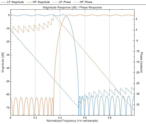
Design two filters. Analyze their magnitude and phase responses using the Filter Analyzer app.

d1 = designfilt("lowpassfir", ...
    PassbandFrequency=0.45,StopbandFrequency=0.55);
d2 = designfilt("highpassfir", ...
    StopbandFrequency=0.35,PassbandFrequency=0.45);

filterAnalyzer(d1,d2,FilterNames=["LP" "HP"], ...
    Analysis="magnitude",OverlayAnalysis="phase")

Analyze Elliptic and FIR Bandpass Filters

Design a tenth-order elliptic bandpass filter with 5 dB of passband ripple and 60 dB of stopband attenuation. Specify passband edge frequencies of $0.2\pi$ rad/sample and $0.45\pi$ rad/sample. Express the design as a cascade of fourth-order transfer functions.

[z,p,k] = ellip(5,5,60,[0.2 0.45]);
[bb,aa] = zp2ctf(z,p,k,SectionOrder=4);

Design a finite impulse response bandpass filter with 5 dB of passband ripple and asymmetric stopbands for use with signals sampled at 2 kHz.

• At lower frequencies, the stopband has 80 dB of attenuation and the transition region ranges from 500 Hz to 600 Hz.

• At higher frequencies, the stopband has 40 dB of attenuation and the transition region ranges from 750 Hz to 900 Hz.

dfir = designfilt("bandpassfir", ...
    SampleRate=2e3,PassbandRipple=5, ...
    StopbandFrequency1=500,PassbandFrequency1=600, ...
    StopbandAttenuation1=80, ...
    PassbandFrequency2=750,StopbandFrequency2=900, ...
    StopbandAttenuation2=40);

Start a Filter Analyzer session to analyze the filters. Import the filters. On the Analyzer tab, click Import Filter.

• To import the elliptic filter, select Filter Coefficients. Select bb as the Numerator and aa as the Denominator. Specify Ellip for the Filter Name, and leave the Sample Rate as Normalized. Click Import.

• To import the FIR filter, select Filter Objects, select dfir, and click Import and Close.

Alternatively, open Filter Analyzer by using the command-line interface. By default, the app displays magnitude responses. Only one of the filters has a sample rate, so the app displays the responses using normalized frequencies.

fa = filterAnalyzer(bb,aa,dfir,FilterNames=["ellip" "dfir"]);

Add a display and use it to plot the magnitude responses and the phase responses of the filters.

• On the Analyzer tab, click New Display.

• Expand the Analysis gallery so the Overlay Analysis section is visible, and click Phase.

• Add the filters by clicking the eye icons on the Filters table.

Alternatively, use the filterAnalysisOptions object and the addDisplays and showFilters functions.

opts = filterAnalysisOptions(OverlayAnalysis="phase");
addDisplays(fa,AnalysisOptions=opts)
showFilters(fa,true,FilterNames=["ellip" "dfir"])

Add another display and show the cumulative magnitude responses of the cascaded transfer functions that specify the elliptic filter.

• Click New Display to add the display and click the eye icon for the elliptic filter.

• On the Display Options tab, click CTF View ▼ and select Cumulative.

Alternatively, use the command-line interface.

addDisplays(fa,CTFAnalysisMode="cumulative")
showFilters(fa,true,FilterNames="ellip")

Add one more display and show the filter specification mask for the FIR filter.

• On the Analyzer tab, click New Display and click the eye icon for the FIR filter. The app displays the frequencies in units of Hz.

• For a digitalFilter object, the app shows the specification mask by default. To remove the mask, on the Display Options tab, click Mask ▼ and clear Specification.

Alternatively, use the command-line interface.

addDisplays(fa)
showFilters(fa,true,FilterNames="dfir")

Impulse and Frequency Response of Halfband Decimation Filter

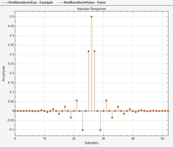
Create two lowpass halfband decimation filters. The design method in the first filter is set to "Equiripple" and in the second filter is set to "Kaiser".

Specify the filter order to be 52. Specify the transition width in normalized frequency units.

filterspec = "Filter order and transition width";
Order = 52;
TW = 0.1859;
firhalfbanddecimEqui = dsp.FIRHalfbandDecimator(...
    NormalizedFrequency=true,...
    Specification=filterspec,...
    FilterOrder=Order,...
    TransitionWidth=TW,...
    DesignMethod="Equiripple");
firhalfbanddecimKaiser = dsp.FIRHalfbandDecimator(...
    NormalizedFrequency=true,......
    Specification=filterspec,...
    FilterOrder=Order,...
    TransitionWidth=TW,...
    DesignMethod="Kaiser");

Plot the impulse response of both the filters. The zeroth-order coefficient is delayed 26 samples, which is equal to the group delay of the filter. This yields a causal halfband filter.

hfvt = filterAnalyzer(firhalfbanddecimEqui,firhalfbanddecimKaiser,...
    Analysis="impulse");
setLegendStrings(hfvt,["Equiripple","Kaiser"])

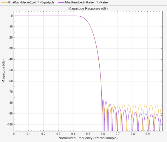
Plot the magnitude and phase response.

If the filter specifications are tight, say a very high filter order with a very narrow transition width, the filter designed using the "Kaiser" method converges more effectively.

hvftMag = filterAnalyzer(firhalfbanddecimEqui,firhalfbanddecimKaiser,...
    Analysis="magnitude");
setLegendStrings(hvftMag,["Equiripple","Kaiser"])

hvftPhase = filterAnalyzer(firhalfbanddecimEqui,firhalfbanddecimKaiser,...
    Analysis="phase");
setLegendStrings(hvftPhase,["Equiripple","Kaiser"])

Version History

Introduced in R2024a

R2025a: Add legend strings and set sample rates

The filterAnalyzer function supports setting legend strings and sample rates.

• The LegendStrings name-value argument enables you to append strings to the default legend strings for all the filters added to Filter Analyzer.

• You can specify a sample rate in the SampleRates name-value argument even if one or more filters are objects with a sample rate.

R2024b: Support for dsp.DCBlocker and dsp.ComplexBandpassDecimator objects

The filterAnalyzer function supports the dsp.DCBlocker and dsp.ComplexBandpassDecimator objects.

R2024b: Support for dsphdl.FIRFilter and dsphdl.BiquadFilter objects

The filterAnalyzer function supports the dsphdl.FIRFilter (DSP HDL Toolbox) and dsphdl.BiquadFilter (DSP HDL Toolbox) objects.