Main Content

designHalfbandIIR

Design and implement halfband IIR filter in the form of a coupled allpass filter

Since R2023b

Description

[a0,a1] = designHalfbandIIR designs a halfband IIR filter in the form of a coupled allpass filter with the filter order of 17 by using the Butterworth design method. The function completes any unspecified design parameters with appropriate default values.

a0 and a1 are the polynomial coefficients of the two allpass filters A0(z) and A1(z). These filters form the two branches of the coupled allpass filter. The transfer function of the IIR halfband filter is given by:

H(z)=0.5*[A0(z2)+z1A1(z2)],

The designHalfbandIIR function implements the allpass filters in the minimum multiplier form. For more information, see Algorithms.

The System object™ argument is false by default. To implement the filter, assign the filter coefficients in a0, a1 to one of the supported System objects.

[a0,a1] = designHalfbandIIR(Name=Value) specifies options using one or more name-value arguments.

For example, [a0,a1] = designHalfbandIIR(FilterOrder=30,TransitionWidth=0.2,DesignMethod="ellip") designs a halfband IIR filter with the filter order of 30 and transition width of 0.2 by using the Elliptic window design method.

When you specify only a partial list of filter parameters, the function designs the filter by setting the other design parameters to their default values.

The function supports two design methods. Each design method supports a specific set of design combinations. For more information, see DesignMethod.

This function supports code generation under certain conditions. For more information, see Code Generation.

example

filtObj = designHalfbandIIR(Name=Value) designs a halfband IIR filter and implements one of the supported System objects.

This syntax applies when you set the SystemObject argument to true.

example

Examples

collapse all

Since R2024a

Design a quasi-linear IIR halfband filter with the order of 32 using the designHalfbandIIR function. Assign the filter coefficients to a coupled allpass filter.

[a0,a1] = designHalfbandIIR(FilterOrder=32,DesignMethod="quasilinphase",Verbose=true)
designHalfbandIIR(FilterOrder=32, TransitionWidth=0.1, DesignMethod="quasilinphase", Structure="single-rate", Datatype="double", SystemObject=false)
a0 = 4×4

     0     0     0     0
     0     0     0     0
     0     0     0     0
     0     0     0     0

a1 = 4×4

         0    0.8085         0    0.3051
         0    0.0387         0    0.2695
         0   -0.7054         0    0.2604
         0    0.3546         0   -0.4386

Construct the corresponding coupled allpass filter using the cascade and parallel functions. Alternatively, if you set the SystemObject argument of the designHalfbandIIR function to true, the function designs the same object.

B0 = dsp.AllpassFilter(AllpassCoefficients=a0);
B1 = dsp.AllpassFilter(AllpassCoefficients=a1);
filtObj = cascade(parallel(B0,cascade(dsp.Delay, B1)),0.5)
filtObj = 
  dsp.FilterCascade with properties:

         Stage1: [1x1 dsp.ParallelFilter]
         Stage2: 0.5000
    CloneStages: true

Create a dsp.DynamicFilterVisualizer object and visualize the magnitude response of the filter.

dfv = dsp.DynamicFilterVisualizer(NormalizedFrequency=true);
dfv(filtObj);

A quasi-linear IIR filter has a fairly constant group delay (hence almost linear phase) in the passband region of the filter.

grpdelay(filtObj)

Figure contains an axes object. The axes object with title Group Delay, xlabel Normalized Frequency ( times pi blank rad/sample), ylabel Group delay (samples) contains an object of type line.

phasez(filtObj)

Figure contains an axes object. The axes object with title Phase Response, xlabel Normalized Frequency ( times pi blank rad/sample), ylabel Phase (radians) contains an object of type line.

Create a spectrumAnalyzer object to visualize the spectra of the input and output signals.

scope = spectrumAnalyzer(SampleRate=2, ...
    PlotAsTwoSidedSpectrum=false,...
    ChannelNames=["Input Signal","Filtered Signal"]);

Stream in a noisy sinusoidal signal and filter the signal using the IIR halfband filter. The sinusoidal tone falls in the passband frequency of the filter and is therefore unaffected.

sine = dsp.SineWave(Frequency=1000,SampleRate=44100,SamplesPerFrame=1024)
sine = 
  dsp.SineWave with properties:

          Amplitude: 1
          Frequency: 1000
        PhaseOffset: 0
      ComplexOutput: false
             Method: 'Trigonometric function'
    SamplesPerFrame: 1024
         SampleRate: 44100
     OutputDataType: 'double'

for i = 1:1000
    x = sine()+0.005*randn(1024,1);
    y = filtObj(x);
    scope(x,y);
end

Design a Butterworth IIR halfband filter with the order of 13 and construct the corresponding coupled allpass filter using the designHalfbandIIR function. Set the SystemObject argument of the function to true.

filtObj = designHalfbandIIR(FilterOrder=13,Verbose=true,SystemObject=true)
designHalfbandIIR(FilterOrder=13, DesignMethod="butter", Structure="single-rate", Datatype="double", SystemObject=true, Passband="lowpass")
filtObj = 
  dsp.FilterCascade with properties:

         Stage1: [1x1 dsp.ParallelFilter]
         Stage2: 0.5000
    CloneStages: true

Create a dsp.DynamicFilterVisualizer object and visualize the magnitude response of the filter.

dfv = dsp.DynamicFilterVisualizer(NormalizedFrequency=true);
dfv(filtObj);

Create a spectrumAnalyzer object to visualize the spectra of the input and output signals.

scope = spectrumAnalyzer(SampleRate=2, ...
    PlotAsTwoSidedSpectrum=false,...
    ChannelNames=["Input Signal","Filtered Signal"]);

Stream in random data and filter the signal using the IIR halfband filter.

for i = 1:1000
    x = randn(1024, 1);
    y = filtObj(x);
    scope(x,y);
end

Design an elliptic IIR halfband decimator object of order 31 and a transition width of 0.1 using the designHalfbandIIR function. Set the Verbose argument to true.

hbIIR = designHalfbandIIR(FilterOrder=31,SystemObject=true,...
    Structure='decim',Verbose=true)
designHalfbandIIR(FilterOrder=31, DesignMethod="butter", Structure="decim", Datatype="double", SystemObject=true, Passband="lowpass")
hbIIR = 
  dsp.IIRHalfbandDecimator with properties:

   Main
                   Specification: 'Coefficients'
                       Structure: 'Minimum multiplier'
              HasPureDelayBranch: false
            AllpassCoefficients1: [8x1 double]
            AllpassCoefficients2: [7x1 double]
    HasTrailingFirstOrderSection: false

  Use get to show all properties

Create a dsp.DynamicFilterVisualizer object and visualize the magnitude response of the filter.

dfv = dsp.DynamicFilterVisualizer(NormalizedFrequency=true,YLimits=[-400 200]);
dfv(hbIIR);

The input is a cosine wave.

Fs = 1;
Fc = 0.03;
input = cos(2*pi*Fc*(0:39)'/Fs);

Decimate the cosine signal using the IIR halfband decimator.

output = hbIIR(input);

Plot the original and decimated signals. In order to plot the two signals in the same plot, you must account for the output delay introduced by the IIR halfband decimator and the scaling introduced by the filter. Use the outputDelay function to compute the delay introduced by the decimator. Shift the output by this delay value.

Visualize the input and the resampled signals. Due to the decimation factor of 2, the output samples coincide with every other input sample.

[delay,FsOut] = outputDelay(hbIIR,FsIn=Fs,Fc=Fc)
delay = 
9.9900
FsOut = 
0.5000
nInput = (0:length(input)-1);
tOutput = (0:length(output)-1)/FsOut-delay;
stem(tOutput,output,'filled',MarkerSize=4); hold on;
stem(nInput,input); hold off;
xlim([-10,25])
legend('Decimated by 2','Input signal','Location','best');

Figure contains an axes object. The axes object contains 2 objects of type stem. These objects represent Decimated by 2, Input signal.

Design an elliptic IIR halfband interpolator object of order 31 and a transition width of 0.1 using the designHalfbandIIR function. Set the Verbose argument to true.

hbIIR = designHalfbandIIR(FilterOrder=31,TransitionWidth=0.1,DesignMethod="ellip",...
    Structure='interp',SystemObject=true,Verbose=true)
designHalfbandIIR(FilterOrder=31, TransitionWidth=0.1, DesignMethod="ellip", Structure="interp", Datatype="double", SystemObject=true, Passband="lowpass")
hbIIR = 
  dsp.IIRHalfbandInterpolator with properties:

                   Specification: 'Coefficients'
             FilterBankInputPort: false
                       Structure: 'Minimum multiplier'
              HasPureDelayBranch: false
            AllpassCoefficients1: [8x1 double]
            AllpassCoefficients2: [7x1 double]
    HasTrailingFirstOrderSection: false

Create a dsp.DynamicFilterVisualizer object and visualize the magnitude response of the filter.

dfv = dsp.DynamicFilterVisualizer(NormalizedFrequency=true);
dfv(hbIIR);

The input is a cosine wave.

Fs = 1;
Fc = 0.08;
input = cos(2*pi*Fc*(0:39)'/Fs);

Interpolate the cosine signal using the IIR halfband interpolator.

output = hbIIR(input);

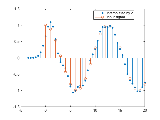
Plot the original and interpolated signals. In order to plot the two signals in the same plot, you must account for the output delay introduced by the IIR halfband interpolator and the scaling introduced by the filter. Use the outputDelay function to compute the delay introduced by the interpolator. Shift the output by this delay value.

Visualize the input and the resampled signals. The input and output values coincide every other sample, due to the interpolation factor of 2.

[delay,FsOut] = outputDelay(hbIIR,FsIn=Fs,Fc=Fc)
delay = 
3.5090
FsOut = 
2
nInput = (0:length(input)-1);
tOutput = (0:length(output)-1)/FsOut-delay;
stem(tOutput,output,'filled',MarkerSize=4); hold on;
stem(nInput,input); hold off;
xlim([-5,20])
legend('Interpolated by 2','Input signal','Location','best');

Figure contains an axes object. The axes object contains 2 objects of type stem. These objects represent Interpolated by 2, Input signal.

Input Arguments

collapse all

Name-Value Arguments

Specify optional pairs of arguments as Name1=Value1,...,NameN=ValueN, where Name is the argument name and Value is the corresponding value. Name-value arguments must appear after other arguments, but the order of the pairs does not matter.

Example: designHalfbandIIR(TransitionWidth=0.1, Passband='highpass',SystemObject=true)

Order of the halfband IIR filter N specified as one of these:

  • 0

  • Odd positive integer greater than 1 when you use the Butterworth or Elliptic design methods

  • Positive integer multiple of 8 when you use the quasi-linear design method (since R2024a)

Data Types: single | double | int8 | int16 | int32 | int64 | uint8 | uint16 | uint32 | uint64

Transition width of the halfband IIR filter, TW, specified as a normalized scalar in the range (0,1].

Data Types: single | double

Stopband attenuation of halfband IIR filter, Ast, specified as a positive scalar.

Data Types: single | double

Window design method, specified as one of these options:

  • 'butter' –– Butterworth design method supports the (N) and (TW,Ast) design specification combinations.

  • 'ellip' –– Elliptic design method supports the (N,TW), (TW,Ast), and (N,Ast) design specification combinations.

  • 'quasilinphase' –– Quasi-linear phase design method supports the (N,TW), (N,Ast), and the (TW,Ast) design specification combinations. (since R2024a)

Data Types: char | string

Option to create System object, specified as:

Data Types: logical

Filter structure, specified as one of these values.

  • 'single-rate' –– When you set SystemObject to:

    • true –– The function returns a coupled allpass filter object comprising of cascaded parallel-structure of dsp.AllpassFilter and dsp.Delay filter objects.

    • false –– The function returns filter coefficients in the form of a0 and a1 matrices.

  • 'interp' –– When you set SystemObject to:

    • true –– The function returns a dsp.IIRHalfbandInterpolator object.

    • false –– The function returns filter coefficients in the form of a0 and a1 matrices.

  • 'decim' –– When you set SystemObject to:

    • true –– The function returns a dsp.IIRHalfbandDecimator object.

    • false –– The function returns filter coefficients in the form of a0 and a1 matrices.

For more information on the dimensions of the coefficient matrices, see the description for a0 and a1 output arguments.

Data Types: char | string

Passband frequency response, specified as one of these:

  • 'lowpass' –– This option supports all three filter structures.

  • 'highpass' –– This option supports only 'single-rate'.

To enable this property, set SystemObject to true.

Data Types: char | string

Option to print the entire function call in MATLAB, specified as one of these:

  • false –– The function does not print the function call.

  • true –– The function prints the entire function call including the default values of the Name=Value arguments that you did not specify when calling the function.

    Use this argument to view all the values used by the function to design and implement the filter.

Data Types: logical

Output Arguments

collapse all

Polynomial coefficients of the first branch of the coupled allpass filter, returned as an N-by-4, N-by-2, or an N-by-1 matrix, where N is the number of filter sections.

The transfer function of the first branch is given by the equation

A0(z)=k=1Nak(0)+z11+ak(0)z1

This table shows the dimensions of the a0 argument for all the design methods and filter structures.

 N'single-rate''interp''decim'
'butter'floor((FilterOrder+1)/4)N-by-2N-by-1N-by-1
'ellip'floor((FilterOrder+1)/4)N-by-2N-by-1N-by-1
'quasilinphase'FilterOrder/4N-by-4N-by-2N-by-2

To return a0, set SystemObject flag to false.

Data Types: double

Polynomial coefficients of the second branch of the coupled allpass filter, returned as an N-by-4, N-by-2, or an N-by-1 matrix. To determine the value of N, see the following table.

The transfer function of the second branch is given by the equation

A1(z)=k=1Nak(1)+z11+ak(1)z1,

This table shows the dimensions of the a1 argument for all the design methods and filter structures:

 'single-rate''interp''decim'
'butter'floor((FilterOrder−1)/4)-by-2floor((FilterOrder−1)/4)-by-1floor((FilterOrder−1)/4)-by-1
'ellip'floor((FilterOrder−1)/4)-by-2floor((FilterOrder−1)/4)-by-1floor((FilterOrder−1)/4)-by-1
'quasilinphase'FilterOrder/4-by-4FilterOrder/4-by-2FilterOrder/4-by-2

To return a1, set SystemObject flag to false.

Data Types: double

Filter object, returned as one of these objects:

To return a filter object, set SystemObject flag to true.

Algorithms

The designHalfbandIIR function models the IIR halfband filter in the form of a coupled allpass filter using the minimum multiplier structure (single-rate implementation) or in the form of an efficient polyphase structure (multirate implementation).

The transfer function of the IIR halfband filter is

H(z)=0.5*[A0(z2)+z1A1(z2)],

The transfer function of A0(z) and A1(z) in the elliptic form is

A0(z)=k=1Nak(0)+z11+ak(0)z1

and

A1(z)=k=1Nak(1)+z11+ak(1)z1,

where N is the number of filter sections of the allpass filters A0(z) and A1(z).

Single-Rate Filter Implementation

When you set Structure to 'single-rate', the designHalfbandIIR function implements a coupled allpass filter object comprising of a cascaded parallel structure of dsp.AllpassFilter and dsp.Delay filter objects.

This is a diagrammatic representation of the filter in the minimum multiplier form when you set Structure to 'single-rate'. The structure of the coupled allpass filter is composed of two allpass filters A0(z) and A1(z) connected in parallel. The designHalfbandIIR function computes the overall filter output by adding the output of the two respective branches.

Input multiplied with a gain of 0.5 goes into two parallel branches A0(z2) and A1(z2). The output from these two branches is added to form the output of the overall filter.

You can design the filters A0(z) and A1(z) using the elliptic design method or the Butterworth design method.

Multirate Filter Implementation

When you set Structure to 'interp' or 'decim', the function implements the filter using an efficient two-branch polyphase structure. For more information on the polyphase implementation, see the Algorithms section in the dsp.IIRHalfbandInterpolator and dsp.IIRHalfbandDecimator object pages.

References

[1] Orfanidis , SJ. High-Order Digital Parametric Equalizer Design. 2005, pp. 1026–46.

Extended Capabilities

Version History

Introduced in R2023b

expand all

Go to top of page