Examine 16-QAM Using MATLAB
This example shows how to process a data stream by using a communications link that consists of a baseband modulator, channel, and demodulator. The example displays a portion of the random data in a stem plot, displays the transmitted and received signals in constellation diagrams, and computes the bit error rate (BER). To add a pulse shaping filter to the communications link, see the Use Pulse Shaping on 16-QAM Signal example. To add forward error correction to the communications link with pulse shape filtering, see the Use Forward Error Correction on 16-QAM Signal example.
Modulate Random Signal
The modulation scheme uses baseband 16-QAM, and the signal passes through an additive white Gaussian noise (AWGN) channel. The basic simulation operations use these Communications Toolbox™ and MATLAB® functions.
rng— Controls the random number generationrandi— Generates a random data streambit2int— Converts the binary data to integer-valued symbolsqammod— Modulates using 16-QAMcomm.AWGNChannel— Impairs the transmitted data using AWGNscatterplot— Creates constellation diagramsqamdemod— Demodulates using 16-QAMint2bit— Converts the integer-valued symbols to binary databiterr— Computes the system BER
Generate Random Binary Data Stream
The conventional format for representing a signal in MATLAB is a vector or matrix. The length of the data stream (that is, the number of rows in the column vector) is arbitrarily set to 30,000. Set the rng function to its default state, or any static seed value, so that the example produces repeatable results. Then use the randi function to generate a column vector containing random values of a binary data stream.
Define parameters.
M = 16;      % Modulation order
k = log2(M); % Number of bits per symbol
n = 30000;   % Number of symbols per frame
sps = 1;     % Number of samples per symbol (oversampling factor)
rng default  % Use default random number generator

dataIn = randi([0 1],n*k,1); % Generate vector of binary data
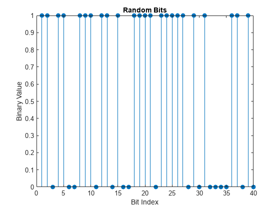
Use a stem plot to show the binary values for the first 40 bits of the random binary data stream. Use the colon (:) operator in the call to the stem function to select a portion of the binary vector.
stem(dataIn(1:40),'filled');
title('Random Bits');
xlabel('Bit Index');
ylabel('Binary Value');
Convert Binary Data to Integer-Valued Symbols
The default configuration for the qammod function expects integer-valued data as the input symbols to modulate. In this example, the binary data stream is preprocessed into integer values before using the qammod function. In particular, the bit2int function converts each 4-tuple to a corresponding integer in the range [0, (M–1)]. The modulation order, M, is 16 in this example.
Perform a bit-to-symbol mapping by specifying the number of bits per symbol defined by . Then, use the bit2int function to convert each 4-tuple to an integer value.
dataSymbolsIn = bit2int(dataIn,k);
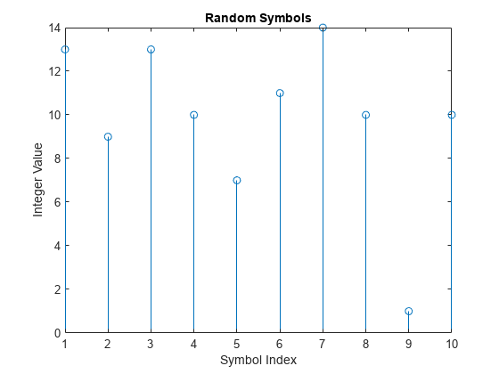
Plot the first 10 symbols in a stem plot.
figure;                    % Create new figure window.
stem(dataSymbolsIn(1:10));
title('Random Symbols');
xlabel('Symbol Index');
ylabel('Integer Value');
Modulate Using 16-QAM
Use the qammod function to apply 16-QAM modulation with phase offset of zero to the dataSymbolsIn column vector for binary-encoded and Gray-encoded bit-to-symbol mappings.
dataMod = qammod(dataSymbolsIn,M,'bin'); % Binary-encoded
dataModG = qammod(dataSymbolsIn,M);      % Gray-encoded
The modulation operation outputs complex column vectors containing values that are elements of the 16-QAM signal constellation. Later in this example constellation diagrams show the binary and Gray symbol mapping.
For more information on modulation functions, see Digital Baseband Modulation. For an example that uses Gray coding with phase-shift keying (PSK) modulation, see Symbol Mapping Examples.
Add White Gaussian Noise
The modulated signal passes through the channel by using the awgn function with the specified signal-to-noise ratio (SNR). Convert the ratio of energy per bit to noise power spectral density () to an SNR value for use by the awgn function. The sps variable is not significant in this example but makes extending the example to use pulse shaping easier. For more information, see the Use Pulse Shaping on 16-QAM Signal example.
Calculate the SNR when the channel has an of 10 dB by using the convertSNR function.
EbNo = 10;
snr = convertSNR(EbNo,'ebno', ...
    samplespersymbol=sps, ...
    bitspersymbol=k);
Pass the signal through the AWGN channel for the binary and Gray coded symbol mappings.
receivedSignal = awgn(dataMod,snr,'measured');
receivedSignalG = awgn(dataModG,snr,'measured');
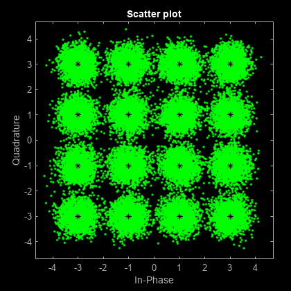
Create Constellation Diagram
Use the scatterplot function to display the in-phase and quadrature components of the modulated signal, dataMod, and the noisy signal received after the channel. The effects of AWGN are present in the constellation diagram.
sPlotFig = scatterplot(receivedSignal,1,0,'g.');
hold on
scatterplot(dataMod,1,0,'k*',sPlotFig)
Demodulate 16-QAM
Use the qamdemod function to demodulate the received data and output integer-valued data symbols.
dataSymbolsOut = qamdemod(receivedSignal,M,'bin'); % Binary-encoded data symbols
dataSymbolsOutG = qamdemod(receivedSignalG,M);     % Gray-coded data symbols
Convert Integer-Valued Symbols to Binary Data
Use the int2bit function to convert the binary-encoded data symbols from the QAM demodulator into a binary vector with length. is the total number of QAM symbols, and is the number of bits per symbol. For 16-QAM, = 4. Repeat the process for the Gray-encoded symbols.
Reverse the bit-to-symbol mapping performed earlier in this example.
dataOut = int2bit(dataSymbolsOut,k);
dataOutG = int2bit(dataSymbolsOutG,k);
Compute System BER
The biterr function calculates the bit error statistics from the original binary data stream, dataIn, and the received data streams, dataOut and dataOutG. Gray coding significantly reduces the BER.
Use the error rate function to compute the error statistics. Use the fprintf function to display the results.
[numErrors,ber] = biterr(dataIn,dataOut);
fprintf('\nThe binary coding bit error rate is %5.2e, based on %d errors.\n', ...
    ber,numErrors)
The binary coding bit error rate is 2.13e-03, based on 255 errors.
[numErrorsG,berG] = biterr(dataIn,dataOutG);
fprintf('\nThe Gray coding bit error rate is %5.2e, based on %d errors.\n', ...
    berG,numErrorsG)
The Gray coding bit error rate is 1.67e-03, based on 200 errors.
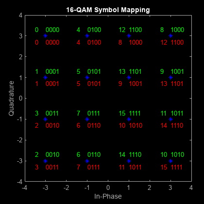
Plot Signal Constellations
The constellation diagram shown previously plotted the points in the QAM constellation, but it did not indicate the mapping between symbol values and the constellation points. In this section, the constellation diagram indicates the mappings for binary-encoding and Gray-encoding of data to constellation points.
Show Natural and Gray Coded Binary Symbol Mapping for 16-QAM Constellation
Apply 16-QAM modulation to complete sets of constellation points by using binary-coded symbol mapping and Gray-coded symbol mapping.
M = 16;                       % Modulation order
x = (0:15);                   % Integer input
symbin = qammod(x,M,'bin');   % 16-QAM output (binary-coded)
symgray = qammod(x,M,'gray'); % 16-QAM output (Gray-coded)
Use the scatterplot function to plot the constellation diagram and annotate it with binary (red) and Gray (green) representations of the constellation points.
scatterplot(symgray,1,0,'b*');
for k = 1:M
    text(real(symgray(k)) - 0.0,imag(symgray(k)) + 0.3, ...
        dec2base(x(k),2,4),'Color',[0 1 0]);
     text(real(symgray(k)) - 0.5,imag(symgray(k)) + 0.3, ...
         num2str(x(k)),'Color',[0 1 0]);

    text(real(symbin(k)) - 0.0,imag(symbin(k)) - 0.3, ...
        dec2base(x(k),2,4),'Color',[1 0 0]);
    text(real(symbin(k)) - 0.5,imag(symbin(k)) - 0.3, ...
        num2str(x(k)),'Color',[1 0 0]);
end
title('16-QAM Symbol Mapping')
axis([-4 4 -4 4])
Examine Plots
Using Gray-coded symbol mapping improves BER performance because the Gray-coded signal constellation points differ by only one bit from each adjacent neighboring point. When using binary-coded symbol mapping, some of the adjacent constellation points differ by two bits. For example, the binary-coded values for 1 (0 0 0 1) and 2 (0 0 1 0) differ by two bits (the third and fourth bits).