yamnet

(Not recommended) YAMNet neural network

Since R2020b

yamnet is not recommended. Use the audioPretrainedNetwork function instead.

Syntax

net = yamnet

Description

net = yamnet returns a pretrained YAMNet model.

This function requires both Audio Toolbox™ and Deep Learning Toolbox™.

Examples

Download YAMNet

Download and unzip the Audio Toolbox™ model for YAMNet.

Type yamnet at the Command Window. If the Audio Toolbox model for YAMNet is not installed, then the function provides a link to the location of the network weights. To download the model, click the link. Unzip the file to a location on the MATLAB path.

Alternatively, execute the following commands to download and unzip the YAMNet model to your temporary directory.

downloadFolder = fullfile(tempdir,'YAMNetDownload');
loc = websave(downloadFolder,'https://ssd.mathworks.com/supportfiles/audio/yamnet.zip');
YAMNetLocation = tempdir;
unzip(loc,YAMNetLocation)
addpath(fullfile(YAMNetLocation,'yamnet'))

Check that the installation is successful by typing yamnet at the Command Window. If the network is installed, then the function returns a SeriesNetwork (Deep Learning Toolbox) object.

yamnet

ans = 
  SeriesNetwork with properties:

         Layers: [86×1 nnet.cnn.layer.Layer]
     InputNames: {'input_1'}
    OutputNames: {'Sound'}

Load Pretrained YAMNet

Load a pretrained YAMNet convolutional neural network and examine the layers and classes.

Use yamnet to load the pretrained YAMNet network. The output net is a SeriesNetwork (Deep Learning Toolbox) object.

net = yamnet

net = 
  SeriesNetwork with properties:

         Layers: [86×1 nnet.cnn.layer.Layer]
     InputNames: {'input_1'}
    OutputNames: {'Sound'}

View the network architecture using the Layers property. The network has 86 layers. There are 28 layers with learnable weights: 27 convolutional layers, and 1 fully connected layer.

net.Layers

ans = 
  86x1 Layer array with layers:

     1   'input_1'                    Image Input              96×64×1 images
     2   'conv2d'                     Convolution              32 3×3×1 convolutions with stride [2  2] and padding 'same'
     3   'b'                          Batch Normalization      Batch normalization with 32 channels
     4   'activation'                 ReLU                     ReLU
     5   'depthwise_conv2d'           Grouped Convolution      32 groups of 1 3×3×1 convolutions with stride [1  1] and padding 'same'
     6   'L11'                        Batch Normalization      Batch normalization with 32 channels
     7   'activation_1'               ReLU                     ReLU
     8   'conv2d_1'                   Convolution              64 1×1×32 convolutions with stride [1  1] and padding 'same'
     9   'L12'                        Batch Normalization      Batch normalization with 64 channels
    10   'activation_2'               ReLU                     ReLU
    11   'depthwise_conv2d_1'         Grouped Convolution      64 groups of 1 3×3×1 convolutions with stride [2  2] and padding 'same'
    12   'L21'                        Batch Normalization      Batch normalization with 64 channels
    13   'activation_3'               ReLU                     ReLU
    14   'conv2d_2'                   Convolution              128 1×1×64 convolutions with stride [1  1] and padding 'same'
    15   'L22'                        Batch Normalization      Batch normalization with 128 channels
    16   'activation_4'               ReLU                     ReLU
    17   'depthwise_conv2d_2'         Grouped Convolution      128 groups of 1 3×3×1 convolutions with stride [1  1] and padding 'same'
    18   'L31'                        Batch Normalization      Batch normalization with 128 channels
    19   'activation_5'               ReLU                     ReLU
    20   'conv2d_3'                   Convolution              128 1×1×128 convolutions with stride [1  1] and padding 'same'
    21   'L32'                        Batch Normalization      Batch normalization with 128 channels
    22   'activation_6'               ReLU                     ReLU
    23   'depthwise_conv2d_3'         Grouped Convolution      128 groups of 1 3×3×1 convolutions with stride [2  2] and padding 'same'
    24   'L41'                        Batch Normalization      Batch normalization with 128 channels
    25   'activation_7'               ReLU                     ReLU
    26   'conv2d_4'                   Convolution              256 1×1×128 convolutions with stride [1  1] and padding 'same'
    27   'L42'                        Batch Normalization      Batch normalization with 256 channels
    28   'activation_8'               ReLU                     ReLU
    29   'depthwise_conv2d_4'         Grouped Convolution      256 groups of 1 3×3×1 convolutions with stride [1  1] and padding 'same'
    30   'L51'                        Batch Normalization      Batch normalization with 256 channels
    31   'activation_9'               ReLU                     ReLU
    32   'conv2d_5'                   Convolution              256 1×1×256 convolutions with stride [1  1] and padding 'same'
    33   'L52'                        Batch Normalization      Batch normalization with 256 channels
    34   'activation_10'              ReLU                     ReLU
    35   'depthwise_conv2d_5'         Grouped Convolution      256 groups of 1 3×3×1 convolutions with stride [2  2] and padding 'same'
    36   'L61'                        Batch Normalization      Batch normalization with 256 channels
    37   'activation_11'              ReLU                     ReLU
    38   'conv2d_6'                   Convolution              512 1×1×256 convolutions with stride [1  1] and padding 'same'
    39   'L62'                        Batch Normalization      Batch normalization with 512 channels
    40   'activation_12'              ReLU                     ReLU
    41   'depthwise_conv2d_6'         Grouped Convolution      512 groups of 1 3×3×1 convolutions with stride [1  1] and padding 'same'
    42   'L71'                        Batch Normalization      Batch normalization with 512 channels
    43   'activation_13'              ReLU                     ReLU
    44   'conv2d_7'                   Convolution              512 1×1×512 convolutions with stride [1  1] and padding 'same'
    45   'L72'                        Batch Normalization      Batch normalization with 512 channels
    46   'activation_14'              ReLU                     ReLU
    47   'depthwise_conv2d_7'         Grouped Convolution      512 groups of 1 3×3×1 convolutions with stride [1  1] and padding 'same'
    48   'L81'                        Batch Normalization      Batch normalization with 512 channels
    49   'activation_15'              ReLU                     ReLU
    50   'conv2d_8'                   Convolution              512 1×1×512 convolutions with stride [1  1] and padding 'same'
    51   'L82'                        Batch Normalization      Batch normalization with 512 channels
    52   'activation_16'              ReLU                     ReLU
    53   'depthwise_conv2d_8'         Grouped Convolution      512 groups of 1 3×3×1 convolutions with stride [1  1] and padding 'same'
    54   'L91'                        Batch Normalization      Batch normalization with 512 channels
    55   'activation_17'              ReLU                     ReLU
    56   'conv2d_9'                   Convolution              512 1×1×512 convolutions with stride [1  1] and padding 'same'
    57   'L92'                        Batch Normalization      Batch normalization with 512 channels
    58   'activation_18'              ReLU                     ReLU
    59   'depthwise_conv2d_9'         Grouped Convolution      512 groups of 1 3×3×1 convolutions with stride [1  1] and padding 'same'
    60   'L101'                       Batch Normalization      Batch normalization with 512 channels
    61   'activation_19'              ReLU                     ReLU
    62   'conv2d_10'                  Convolution              512 1×1×512 convolutions with stride [1  1] and padding 'same'
    63   'L102'                       Batch Normalization      Batch normalization with 512 channels
    64   'activation_20'              ReLU                     ReLU
    65   'depthwise_conv2d_10'        Grouped Convolution      512 groups of 1 3×3×1 convolutions with stride [1  1] and padding 'same'
    66   'L111'                       Batch Normalization      Batch normalization with 512 channels
    67   'activation_21'              ReLU                     ReLU
    68   'conv2d_11'                  Convolution              512 1×1×512 convolutions with stride [1  1] and padding 'same'
    69   'L112'                       Batch Normalization      Batch normalization with 512 channels
    70   'activation_22'              ReLU                     ReLU
    71   'depthwise_conv2d_11'        Grouped Convolution      512 groups of 1 3×3×1 convolutions with stride [2  2] and padding 'same'
    72   'L121'                       Batch Normalization      Batch normalization with 512 channels
    73   'activation_23'              ReLU                     ReLU
    74   'conv2d_12'                  Convolution              1024 1×1×512 convolutions with stride [1  1] and padding 'same'
    75   'L122'                       Batch Normalization      Batch normalization with 1024 channels
    76   'activation_24'              ReLU                     ReLU
    77   'depthwise_conv2d_12'        Grouped Convolution      1024 groups of 1 3×3×1 convolutions with stride [1  1] and padding 'same'
    78   'L131'                       Batch Normalization      Batch normalization with 1024 channels
    79   'activation_25'              ReLU                     ReLU
    80   'conv2d_13'                  Convolution              1024 1×1×1024 convolutions with stride [1  1] and padding 'same'
    81   'L132'                       Batch Normalization      Batch normalization with 1024 channels
    82   'activation_26'              ReLU                     ReLU
    83   'global_average_pooling2d'   Global Average Pooling   Global average pooling
    84   'dense'                      Fully Connected          521 fully connected layer
    85   'softmax'                    Softmax                  softmax
    86   'Sound'                      Classification Output    crossentropyex with 'Speech' and 520 other classes

To view the names of the classes learned by the network, you can view the Classes property of the classification output layer (the final layer). View the first 10 classes by specifying the first 10 elements.

net.Layers(end).Classes(1:10)

ans = 10×1 categorical
     Speech 
     Child speech, kid speaking 
     Conversation 
     Narration, monologue 
     Babbling 
     Speech synthesizer 
     Shout 
     Bellow 
     Whoop 
     Yell 

Use analyzeNetwork (Deep Learning Toolbox) to visually explore the network.

analyzeNetwork(net)

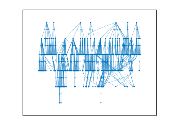
YAMNet was released with a corresponding sound class ontology, which you can explore using the yamnetGraph object.

ygraph = yamnetGraph;
p = plot(ygraph);
layout(p,'layered')

The ontology graph plots all 521 possible sound classes. Plot a subgraph of the sounds related to respiratory sounds.

allRespiratorySounds = dfsearch(ygraph,"Respiratory sounds");
ygraphSpeech = subgraph(ygraph,allRespiratorySounds);
plot(ygraphSpeech)

Classify Sounds Using YAMNet

Read in an audio signal to classify it.

[audioIn,fs] = audioread("TrainWhistle-16-44p1-mono-9secs.wav");

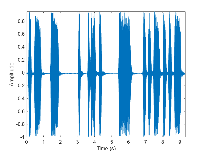
Plot and listen to the audio signal.

t = (0:numel(audioIn)-1)/fs;
plot(t,audioIn)
xlabel("Time (s)")
ylabel("Ampltiude")
axis tight

sound(audioIn,fs)

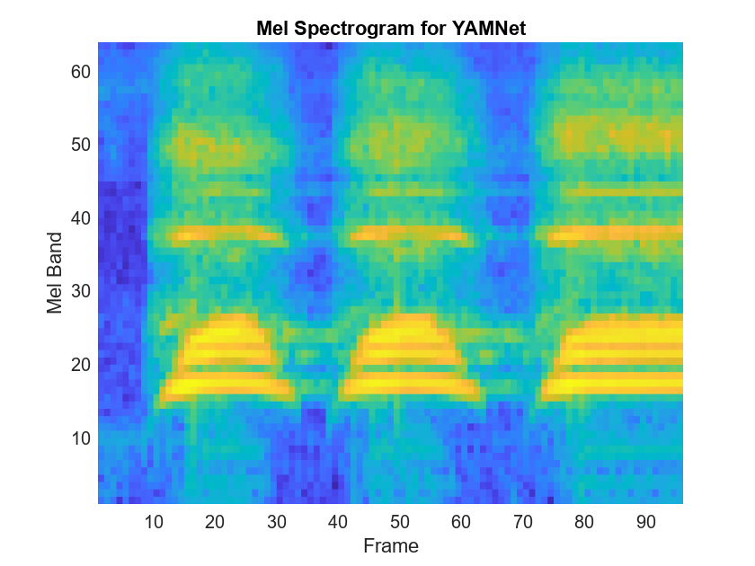
YAMNet requires you to preprocess the audio signal to match the input format used to train the network. The preprocesssing steps include resampling the audio signal and computing an array of mel spectrograms. To learn more about mel spectrograms, see melSpectrogram. Use yamnetPreprocess to preprocess the signal and extract the mel spectrograms to be passed to YAMNet. Visualize one of these spectrograms chosen at random.

spectrograms = yamnetPreprocess(audioIn,fs);

arbitrarySpect = spectrograms(:,:,1,randi(size(spectrograms,4)));
surf(arbitrarySpect,EdgeColor="none")
view([90 -90])
xlabel("Mel Band")
ylabel("Frame")
title("Mel Spectrogram for YAMNet")
axis tight

Create a YAMNet neural network using the audioPretrainedNetwork function. Call predict with the network on the preprocessed mel spectrogram images. Convert the network output to class labels using scores2label.

[net,classNames] = audioPretrainedNetwork("yamnet");
scores = predict(net,spectrograms);
classes = scores2label(scores,classNames);

The classification step returns a label for each of the spectrogram images in the input. Classify the sound as the most frequently occurring label in the output.

mySound = mode(classes)

mySound = categorical
     Whistle 

Transfer Learning Using YAMNet

Download and unzip the air compressor data set [1]. This data set consists of recordings from air compressors in a healthy state or one of 7 faulty states.

url = "https://www.mathworks.com/supportfiles/audio/AirCompressorDataset/AirCompressorDataset.zip";
downloadFolder = fullfile(tempdir,"aircompressordataset");
datasetLocation = tempdir;

if ~exist(fullfile(tempdir,"AirCompressorDataSet"),"dir")
    loc = websave(downloadFolder,url);
    unzip(loc,fullfile(tempdir,"AirCompressorDataSet"))
end

Create an audioDatastore object to manage the data and split it into train and validation sets.

ads = audioDatastore(downloadFolder,IncludeSubfolders=true,LabelSource="foldernames");

[adsTrain,adsValidation] = splitEachLabel(ads,0.8,0.2);

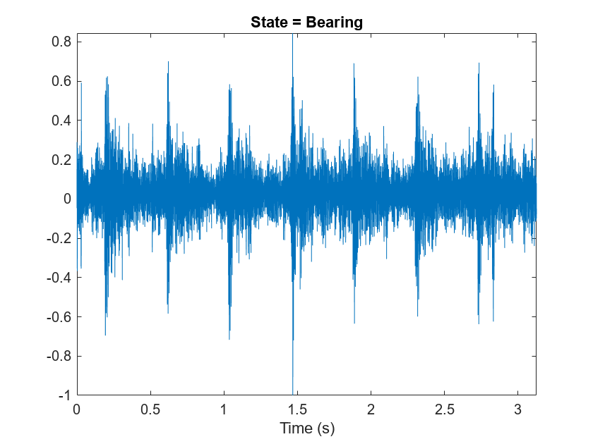
Read an audio file from the datastore and save the sample rate for later use. Reset the datastore to return the read pointer to the beginning of the data set. Listen to the audio signal and plot the signal in the time domain.

[x,fileInfo] = read(adsTrain);
fs = fileInfo.SampleRate;

reset(adsTrain)

sound(x,fs)

figure
t = (0:size(x,1)-1)/fs;
plot(t,x)
xlabel("Time (s)")
title("State = " + string(fileInfo.Label))
axis tight

Extract Mel spectrograms from the train set using yamnetPreprocess. There are multiple spectrograms for each audio signal. Replicate the labels so that they are in one-to-one correspondence with the spectrograms.

emptyLabelVector = adsTrain.Labels;
emptyLabelVector(:) = [];

trainFeatures = [];
trainLabels = emptyLabelVector;
while hasdata(adsTrain)
    [audioIn,fileInfo] = read(adsTrain);
    features = yamnetPreprocess(audioIn,fileInfo.SampleRate);
    numSpectrums = size(features,4);
    trainFeatures = cat(4,trainFeatures,features);
    trainLabels = cat(2,trainLabels,repmat(fileInfo.Label,1,numSpectrums));
end

Extract features from the validation set and replicate the labels.

validationFeatures = [];
validationLabels = emptyLabelVector;
while hasdata(adsValidation)
    [audioIn,fileInfo] = read(adsValidation);
    features = yamnetPreprocess(audioIn,fileInfo.SampleRate);
    numSpectrums = size(features,4);
    validationFeatures = cat(4,validationFeatures,features);
    validationLabels = cat(2,validationLabels,repmat(fileInfo.Label,1,numSpectrums));
end

The air compressor data set has only 8 classes. Call audioPretrainedNetwork with NumClasses set to 8 to load a pretrained YAMNet network with the desired number of output classes for transfer learning.

classNames = unique(adsTrain.Labels);
numClasses = numel(classNames);

net = audioPretrainedNetwork("yamnet",NumClasses=numClasses);

To define training options, use trainingOptions.

miniBatchSize = 128;
validationFrequency = floor(numel(trainLabels)/miniBatchSize);
options = trainingOptions('adam', ...
    InitialLearnRate=3e-4, ...
    MaxEpochs=2, ...
    MiniBatchSize=miniBatchSize, ...
    Shuffle="every-epoch", ...
    Plots="training-progress", ...
    Metrics="accuracy", ...
    Verbose=false, ...
    ValidationData={single(validationFeatures),validationLabels'}, ...
    ValidationFrequency=validationFrequency);

To train the network, use trainnet.

airCompressorNet = trainnet(trainFeatures,trainLabels',net,"crossentropy",options);

Save the trained network to airCompressorNet.mat. You can now use this pre-trained network by loading the airCompressorNet.mat file.

save airCompressorNet.mat airCompressorNet 

References

[1] Verma, Nishchal K., et al. “Intelligent Condition Based Monitoring Using Acoustic Signals for Air Compressors.” IEEE Transactions on Reliability, vol. 65, no. 1, Mar. 2016, pp. 291–309. DOI.org (Crossref), doi:10.1109/TR.2015.2459684.

Output Arguments

net — Pretrained YAMNet neural network

SeriesNetwork object

Pretrained YAMNet neural network, returned as a SeriesNetwork (Deep Learning Toolbox) object.

References

[1] Gemmeke, Jort F., et al. “Audio Set: An Ontology and Human-Labeled Dataset for Audio Events.” 2017 IEEE International Conference on Acoustics, Speech and Signal Processing (ICASSP), IEEE, 2017, pp. 776–80. DOI.org (Crossref), doi:10.1109/ICASSP.2017.7952261.

[2] Hershey, Shawn, et al. “CNN Architectures for Large-Scale Audio Classification.” 2017 IEEE International Conference on Acoustics, Speech and Signal Processing (ICASSP), IEEE, 2017, pp. 131–35. DOI.org (Crossref), doi:10.1109/ICASSP.2017.7952132.

Extended Capabilities

C/C++ Code Generation

Generate C and C++ code using MATLAB® Coder™.

Usage notes and limitations:

• To create a SeriesNetwork or DAGNetwork object for code generation, see Load Pretrained Networks for Code Generation (MATLAB Coder).

GPU Code Generation

Generate CUDA® code for NVIDIA® GPUs using GPU Coder™.

Usage notes and limitations:

• To create a SeriesNetwork or DAGNetwork object for code generation, see Load Pretrained Networks for Code Generation (GPU Coder).

Version History

Introduced in R2020b