OptimizerTRSADEA
Description
Use the OptimizerTRSADEA object to create a TR-SADEA optimizer. Use
the object's properties and functions to set up and tune the optimizer parameters. Then,
integrate the TR-SADEA optimizer as a black box into your workflow using a function
handle.
You can use the TR-SADEA optimizer for high-dimensional (with 30 or more design variables), highly nonlinear problems where focused local search and adaptive refinement is necessary. It is particularly effective for applications such as optimizing large-scale antenna arrays (phased arrays, MIMO antennas, or reconfigurable metasurfaces), high-fidelity EM simulations with many constraints, and fine-tuning near an optimal design.
The TR-SADEA optimizer aims to find a global minimum of the objective function across several design variables within a bounded domain. For more information, see Antenna and Array Optimization Algorithms.
Creation
Description
s = OptimizerTRSADEA(bounds)bounds.
s = OptimizerTRSADEA(bounds,PropertyName=Value)PropertyName is the property
name and Value is the corresponding value. You can specify the
name-value arguments in any order as
PropertyName1=Value1,...,PropertyNameN=ValueN. Properties that you
do not specify retain their default values.
For example, s = OptimizerTRSADEA([1;3],UseParallel=1) creates a
TR-SADEA optimizer object with a single design variable with a lower bound of 1 and
upper bound of 3 and uses a parallel pool for optimization.
Input Arguments
Properties
Object Functions
checkExitCondition | Check exit status of optimizer |
defineInitialPopulation | Set initial population size |
getBestMemberData | View best member data after optimization |
getInitializationData | View optimizer member data at initialization |
getIterationData | View optimization data for completed iterations |
getNumberOfEvaluations | Get number of function evaluations performed |
isConverged | Check convergence status of optimizer |
isFunctionEvaluationsExhausted | Check function evaluations completion status |
optimize | Optimize custom evaluation function using specified parameters |
optimizeWithPlots | Optimize custom evaluation function and plot population density and convergence |
performRestore | Restore optimizer parameters to values from the previous successful iteration |
setMaxFunctionEvaluations | Set upper limit for number of function evaluations |
showConvergenceTrend | Plot optimization convergence trend |
validateSetup | Validate optimizer setup |
Examples
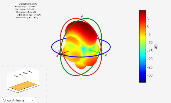
Create a four-element linear array of dipole antennas. Use it as an exciter for a reflector antenna.
Calculate maximum directivity of this reflector antenna.
freq = 70e6;
la = linearArray(NumElements=4);
la.Tilt = 90;
referenceAnt = reflector;
referenceAnt.Exciter = la;
referenceAnt.GroundPlaneLength = 8;
referenceAnt.GroundPlaneWidth = 4;
referenceAnt.Spacing = 4;
InitialDirectivity = max(max(pattern(referenceAnt,freq)))
InitialDirectivity =
9.9029
figure
pattern(referenceAnt,freq)
Find the lowest return loss among all ports of this antenna at 70 MHz.
sp = sparameters(referenceAnt,freq);
RetLossPort1 = 20*log10(max(abs(rfparam(sp,1,1))));
RetLossPort2 = 20*log10(max(abs(rfparam(sp,2,2))));
RetLossPort3 = 20*log10(max(abs(rfparam(sp,3,3))));
RetLossPort4 = 20*log10(max(abs(rfparam(sp,4,4))));
InitialLowestRetLossVal = max([RetLossPort1,RetLossPort2,RetLossPort3,RetLossPort4]);
Choose spacing between the dipoles of the exciter and exciter to reflector spacing as design variables. Specify the lower and upper bounds of these design variables.
Use the TR-SADEA optimizer to optimize this reflector antenna for its directivity and return loss. Specify an evaluation function for optimization using the CustomEvaluationFunction property of the OptimizerTRSADEA object. The evaluation function used in this example is defined at the end of this example.
Set the maximum number of function evaluations to 90 and initial population sample size to 10. Setting these parameters is optional. The TR-SADEA optimizer calculates best sample size automatically if you do not specify it.
Bounds = [0.1 0.1; 10 10];
s = OptimizerTRSADEA(Bounds);
s.CustomEvaluationFunction = @customEvaluationWithConstraint2;
setMaxFunctionEvaluations(s,90);
defineInitialPopulation(s,10);
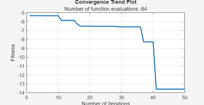
Validate the optimizer setup. Run the optimization for 50 iterations and check if maximum function evaluations have been reached. Observe the convergence trends plot.
validateSetup(s)
ans = logical
   1
optimize(s,50);
flag0 = isFunctionEvaluationsExhausted(s)
flag0 = logical
   0
showConvergenceTrend(s)
View the best member data.
bestDesign = s.getBestMemberData
bestDesign =
  bestMemberData with properties:

             member: [7.6028 5.3499]
       performances: -6.4699
            fitness: -6.4699
    bestIterationId: 47
bestDesignValues = bestDesign.member
bestDesignValues = 1×2

    7.6028    5.3499
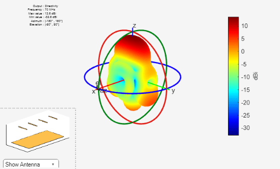
Update the reference antenna with design values obtained from the optimization and calculate the directivity.
Observe the increase in directivity post optimization.
referenceAnt.Exciter.ElementSpacing = bestDesignValues(1);
referenceAnt.Spacing = bestDesignValues(2);
postOptimizationDirectivity = max(max(pattern(referenceAnt,freq)))
postOptimizationDirectivity =
11.4678
figure
pattern(referenceAnt,freq)
Calculate the post optimization return loss. Use the lowest return loss value among all ports.
Observe that the value of return loss after optimization is better than its previous value.
sp = sparameters(referenceAnt,freq);
RetLossPort1 = 20*log10(max(abs(rfparam(sp,1,1))));
RetLossPort2 = 20*log10(max(abs(rfparam(sp,2,2))));
RetLossPort3 = 20*log10(max(abs(rfparam(sp,3,3))));
RetLossPort4 = 20*log10(max(abs(rfparam(sp,4,4))));
NewLowestRetLossVal = max([RetLossPort1,RetLossPort2,RetLossPort3,RetLossPort4]);
Check the exit status of the optimizer.
flag1 = isFunctionEvaluationsExhausted(s)
flag1 = logical
   0
flag2 = checkExitCondition(s)
flag2 = logical
   0
Restore the optimizer parameters to their previous successful iteration values. Use this step if the current iteration is interrupted and the iteration data is incomplete.
res = performRestore(s)
res =
  OptimizerTRSADEA with properties:

                      Bounds: [2×2 double]
    CustomEvaluationFunction: @customEvaluationWithConstraint2
                     Weights: []
                 UseParallel: 0
        GeometricConstraints: [1×1 struct]
                   EnableLog: 0
This code defines the evaluation function used in this example.
function fitness = customEvaluationWithConstraint2(designVariables)

        % Create geometry
        la = linearArray(NumElements=4);
        la.Tilt = 90;
        la.ElementSpacing = designVariables(1);
        r = reflector;
        r.Exciter = la;
        r.GroundPlaneLength = 8;
        r.GroundPlaneWidth = 4;
        r.Spacing = designVariables(2);

        % Calculate realized gain
        objective = max(max(pattern(r, 70e6)));
        objective = -objective; % As optimizer always minimizes objective,
        % sign is reversed to maximize gain.

        % Constraints s11 < -10
        % Calculate S-parameters
        freq = 70e6;
        s = sparameters(r,freq);
        RetLossPort1 = 20*log10(max(abs(rfparam(s,1,1))));
        RetLossPort2 = 20*log10(max(abs(rfparam(s,2,2))));
        RetLossPort3 = 20*log10(max(abs(rfparam(s,3,3))));
        RetLossPort4 = 20*log10(max(abs(rfparam(s,4,4))));
        lowestRetLossVal = max([RetLossPort1,RetLossPort2,RetLossPort3,RetLossPort4]);
        expVal = -20;

        % As constraint is satisfied when it is less than -20 dB, better
        % values are made to be equal to -20 dB to not affect optimizer
        % direction.
        constraint = (lowestRetLossVal-expVal);
        constraint = max(constraint,0);

        % Handle errors during S-parameters computation.
        % High penalty value is used to handle errors.
        fitness = objective + constraint;

end