Analyze Dynamic Response and Flying Qualities of Aerospace Vehicles
Aerospace Blockset™ provides flight control analysis tools that you can use to analyze the dynamic response and flying qualities of aerospace vehicles.
Flight Control Analysis Live Scripts — MATLAB® live scripts demonstrate dynamic response and flying quality analysis of Sky Hogg and de Havilland Beaver airframes.
Modify Flight Control Analysis Templates — You can use templates to analyze the flying qualities of three degree-of-freedom and six degree-of-freedom airframe models. When you are comfortable running the analysis on the default airframes, you can replace them with your own airframe and analyze it.
Plot Short-Period Undamped Natural Frequency Results — After computing lateral-directional handling qualities, use the Aerospace Toolbox short-period functions to plot the short-period undamped natural frequency response.
Note
Analyzing dynamic response and flying qualities of airframes requires a Simulink® Control Design™ license.
Flight Control Analysis Live Scripts
Each flight control analysis template has an associated MATLAB live script that guides you through a flying quality analysis workflow for the default airframe. You can interact with the script and explore the analysis workflow.
Flying Quality Analysis for 6DOF De Havilland Beaver Airframe — Compute longitudinal and lateral-directional flying qualities for a De Havilland Beaver airframe.
Longitudinal Flying Quality Analysis for 3DOF Sky Hogg Longitudinal Airframe — Compute longitudinal flying qualities for a Sky Hogg airframe.
For more information on running live scripts, see Create and Run Sections in Code.
Open , a 6DOF template. For example,
asbFlightControlAnalysis('6DOF')Navigate to the Getting Started section and click the first link.
Alternatively, enter this command in the Command Window.
openExample('aeroblks/FlyingQuality6DOFAnalysisExample')The script describes how to use eigenvalue analysis to determine the longitudinal flying qualities (long-period phugoid mode and short-period mode) and lateral-directional flying qualities (Dutch roll mode, roll mode, and spiral mode) for an aircraft modeled in Simulink.
As you run the script, when applicable, the results of the runs display inline.
Modify Flight Analysis Templates
Aerospace Blockset provides these templates:
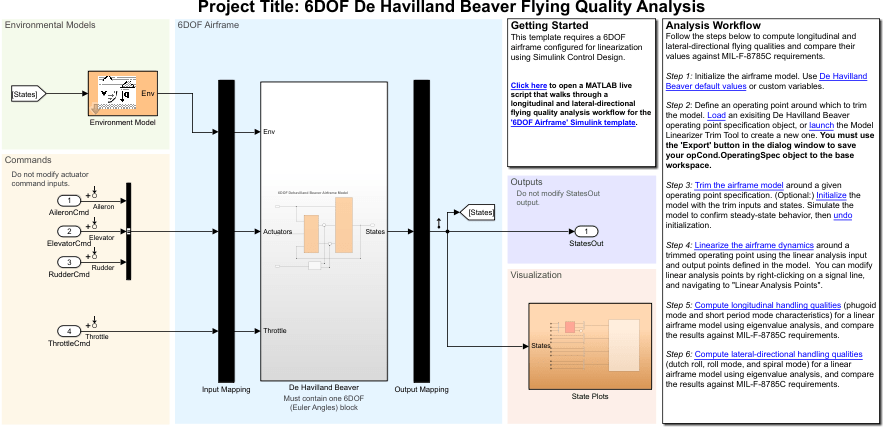
6DOF De Havilland Beaver Flying Quality Analysis— At the MATLAB command line, typeasbFlightControlAnalysis('6DOF','flightControl6DOFAirframeTemplate'). This template uses a six degree-of-freedom airframe configured for linearization and quality analysis. For initialization, the template uses the de Havilland Beaver airframe parameters.3DOF Sky Hogg Longitudinal Flying Quality Analysis— At the MATLAB command line, typeasbFlightControlAnalysis('3DOF','flightControl3DOFAirframeTemplate'). This template uses a three degree-of-freedom longitudinal airframe configured for linearization and quality analysis. For initialization, the template uses Sky Hogg airframe parameters.
When you are comfortable navigating the flight control analysis templates with the default airframes, consider customizing the templates for your own airframe model.
Flight Control Analysis Templates
To familiarize yourself with Aerospace Blockset flight control analysis templates:
Open a template. For example, to open a 3DOF template, enter this command:
asbFlightControlAnalysis('3DOF')To open a 6DOF template, enter this command:
asbFlightControlAnalysis('6DOF')The flight control analysis model opens.

The Analysis Workflow section contains a clickable guided workflow to compute longitudinal and lateral-directional flying qualities and compare their values against MIL-F-8785C requirements. Each step creates the necessary variables for the step. To perform the flying quality analysis, sequentially click the links in the steps.
Create an operating point specification object in the base workspace for the airframe model using the Model Linearizer. Alternatively, load the default object provided in step 2.
To trim the airframe, click Trim the airframe in step 3. This action calls the
trimAirframefunction.To linearize the airframe around a trimmed operating point, click Linearize the airframe in step 4. This action calls the
linearizeAirframefunction.To compute the longitudinal flying qualities, click Compute longitudinal handling qualities. This action calls the
computeLongitudinalFlyingQualitiesfunction.To compute the lateral-directional handling qualities, click Compute lateral-directional handling qualities in step 6. This action calls the
computeLateralDirectionalFlyingQualitiesfunction.
Modify Flight Control Analysis Templates
When you are comfortable using the 3DOF and 6DOF flight control analysis templates to trim, linearize, and compute the longitudinal and lateral-directional handling qualities for the default airframes, consider customizing the templates to include your own airframe.
Open a 3DOF or 6DOF template and change the airframe to one of your own. For example, to change the template airframe to an external model, enter this command.
asbFlightControlAnalysis('6DOF','sixDOFAirframeExample','DehavillandBeaver6DOFAirframe')This command replaces the de Havilland Beaver subsystem with the
DehavillandBeaver6DOFAirframemodel and includes it as a referenced model.
Alternatively, in the corresponding canvas, manually replace the default model airframe in the blue area with your own airframe.
On the canvas, align the inputs and outputs of the airframe using the Input Mapping and Output Mapping subsystems.
Create a new operating point specification object. In the Analysis Workflow section, go to step 2 and start the Model Linearizer by clicking Launch.
To save your
opCond.OperatingSpecobject to the base workspace, click Export in the dialog window.To trim, linearize, and compute the longitudinal and lateral-directional handling qualities for the airframe model, click the links in workflow steps 3, 4, 5, and 6.
Explore Flight Control Analysis Functions
The flight control analysis live scripts and template workflows use these functions:
asbFlightControlAnalysistrimAirframelinearizeAirframecomputeLongitudinalFlyingQualitiescomputeLateralDirectionalFlyingQualities
To customize your own scripts to trim airframes around operating points, linearize airframes, and calculate longitudinal and lateral-directional handling qualities, you can use these functions in a workflow:
Create a flight control analysis template using the
asbFlightControlAnalysisfunction.Trim the airframe model around an operating point using the
trimAirframefunction.This step creates a trimmed operating point, which the
linearizeAirframefunction requires.Linearize the airframe model around the trimmed operating point using the
linearizeAirframefunction.This step creates a state space model that describes the linearized dynamics of the airframe model at a trimmed operating point.
Compute the flying qualities for the airframe, including short- and long-period (phugoid) mode characteristics of the specified state space model, using the
computeLongitudinalFlyingQualitiesfunction. Compute lateral-directional (Dutch roll, roll, and spiral) mode characteristics, using thecomputeLateralDirectionalFlyingQualitiesfunction.
This code shows an example workflow using these functions.
asbFlightControlAnalysis('6DOF','DehavillandBeaverAnalysisModel');
opSpecDefault = DehavillandBeaver6DOFOpSpec('DehavillandBeaverAnalysisModel');
opTrim = trimAirframe('DehavillandBeaverAnalysisModel',opSpecDefault);
linSys = linearizeAirframe('DehavillandBeaverAnalysisModel',opTrim);
lonFlyingQual = computeLongitudinalFlyingQualities('DehavillandBeaverAnalysisModel',linSys)
latFlyingQual = computeLateralDirectionalFlyingQualities('DehavillandBeaverAnalysisModel',linSys)
Plot Short-Period Undamped Natural Frequency Results
After computing the lateral-directional handling qualities, you can
plot the short-period undamped natural frequency response ωnSP
using the shortPeriodCategoryAPlot function. To plot the category B or category
C flight phase, use the shortPeriodCategoryBPlot or shortPeriodCategoryCPlot function. This example describes how to plot
the short-period undamped natural frequency response for the Sky Hogg model.
Start the flight control analysis template for the 3DOF configuration.
asbFlightControlAnalysis('3DOF')The
3DOF Sky Hogg Longitudinal Flying Quality Analysisproject starts in the Simulink Editor.To compute longitudinal and lateral-directional flying qualities, in the Analysis Workflow section, click through the guided workflow. Click OK when prompted.
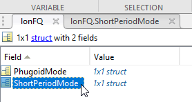
After computing longitudinal and lateral-directional flying qualities, find and double-click the
lonFQstructure in your workspace.
In the variables viewer, double-click the
ShortPeriodModevariable.
Check that the
wnvariable exists. Thewnvariable is the short-period undamped natural frequency response you want to plot.Plot the short-period undamped natural frequency response. In the MATLAB Command Window, use the
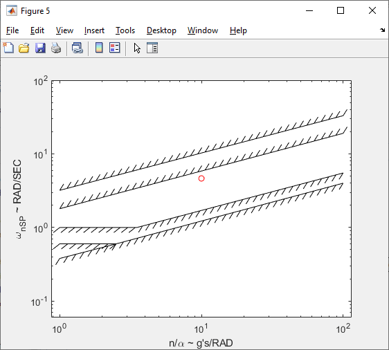
shortPeriodCategoryAPlotfunction. For example, for a load factor per angle of attack of10, enter this command.shortPeriodCategoryAPlot(10, lonFQ.ShortPeriodMode.wn, 'ro')A figure window with the plotted short-period undamped natural frequency response opens.

To evaluate if the results are within your tolerance limits, check that the red dot is within your limits.
See Also
asbFlightControlAnalysis | computeLateralDirectionalFlyingQualities | computeLongitudinalFlyingQualities | linearizeAirframe | trimAirframe | shortPeriodCategoryAPlot | shortPeriodCategoryBPlot | shortPeriodCategoryCPlot | Model Linearizer (Simulink Control Design)