Lidar Camera Calibration and Fusion

This example shows how to estimate the rigid transformation between a lidar sensor and a camera, and how to use the calibration results to fuse the point cloud data from the lidar sensor and the image data from the camera.

Overview

Lidar sensors and cameras are often used together because they provide complementary information. Lidar sensors capture 3-D spatial data, while cameras capture images that include more information about appearance and texture. By fusing data from both sensors, you can enhance object detection and classification workflows. Lidar camera calibration estimates a transformation matrix that describes the relative rotation and translation of the lidar sensor with respect to the camera. This transformation can be used to fuse lidar and camera data.

This diagram illustrates the workflow for lidar camera calibration. The process begins by using a calibration board, such as a checkerboard, ChArUco board, or AprilGrid, and by capturing multiple frames where the board is visible in both the point clouds and the images. Next, you detect the calibration board in both the point clouds and the images, and estimate the board corners in the lidar and camera coordinate frames. The left side of the diagram shows a point cloud with its detected calibration board in the Lidar coordinate frame, and the right side of the diagram shows the detected calibration board in the camera frame. Calibration outputs the rigid transformation that aligns the board corners in the Lidar coordinate frame to the board corners in the camera coordinate frame, represented as a rigidtform3d object. For more information on lidar camera calibration, see What Is Lidar-Camera Calibration?

This example uses a synchronized pair of PNG images and PCD point clouds collected with an Ouster OS1 lidar sensor. It assumes that you already estimated the intrinsic parameters of the camera. For more information on computing camera intrinsics, see Evaluating the Accuracy of Single Camera Calibration.

Load Calibration Data

Load images and point cloud data into the workspace.

imageDataPath = fullfile(toolboxdir("lidar"),"lidardata","calibration","images");
imds = imageDatastore(imageDataPath);
imageFileNames = imds.Files;

ptCloudFilePath = fullfile(toolboxdir("lidar"),"lidardata","calibration","pointClouds");
pcds = fileDatastore(ptCloudFilePath,ReadFcn=@pcread);
ptCloudFileNames = pcds.Files;

Load camera intrinsics into the workspace.

cameraIntrinsicFile = fullfile(imageDataPath,"intrinsics.mat");
intrinsics = load(cameraIntrinsicFile).intrinsics;

Detect Board Corners in Images

Disable the warning for symmetric board usage. While symmetric boards are not recommended, the uniform padding and the limited board rotation (less than 45 degrees in the collected images) ensure that symmetry does not affect the results.

currentState = warning;
warning("off","vision:calibrate:boardShouldBeAsymmetric")

Detect the checkerboard points.

[imagePoints,patternDims] = detectCheckerboardPoints(imageFileNames,PartialDetections=false);

Restore the original warning state.

warning(currentState)

Specify the checkerboard parameters according to the following diagram.

Specify the square size in millimeters.

squareSize = 100;

Specify the padding [P1 P2 P3 P4] in millimeters.

padding = [100 100 100 100];

Estimate the board corners in the camera coordinate frame.

[cornersCamera,boardSize] = estimateBoardCornersCamera("checkerboard",imagePoints,...
    intrinsics,patternDims,squareSize,Padding=padding);

Visualize all the detected boards in the camera frame.

figure
cam = plotCamera(Size=0.25,Opacity=0.8);
hold on

numImages = numel(imageFileNames);
plotColors = hsv(numImages);
cornerIdx = [1 2 3 4 1];
for i = 1:numImages
    plot3(cornersCamera(cornerIdx,1,i),cornersCamera(cornerIdx,2,i),cornersCamera(cornerIdx,3,i),Color=plotColors(i,:),LineWidth=2)
end
set(gca,CameraUpVector=[-1 0 0]);

Detect Board Corners in Point Clouds

Preprocess the point cloud by first selecting the region of interest to speed up detection and then removing the ground points.

roi = [-5 5 -Inf Inf -Inf Inf];

numPtClouds = numel(ptCloudFileNames);
ptCloudArr = repmat(pointCloud(zeros(0,3)),numPtClouds,1);

for i = 1:numPtClouds
    ptCloud = pcread(ptCloudFileNames{i});

    idx = findPointsInROI(ptCloud,roi);
    ptCloud = select(ptCloud,idx);

    [~,ptCloud] = segmentGroundSMRF(ptCloud,MaxWindowRadius=8,ElevationThreshold=0.2,ElevationScale=1.25);

    ptCloudArr(i) = ptCloud;
end

Specify the cluster threshold to cluster each point cloud for board detection.

clusterThreshold = 0.05;

Specify the plane fitting distance used to fit a plane to each point cloud cluster for board detection.

planeFitDistance = 0.05;

Estimate the board corners in the lidar frame.

[cornersLidar,ptCloudBoard] = estimateBoardCornersLidar(ptCloudArr,clusterThreshold,boardSize,...
    PlaneFitDistance=planeFitDistance);

Visualize all the detected calibration boards in the lidar frame.

figure
allPtClouds = pccat(ptCloudArr);
pcshow(allPtClouds)
hold on

for i = 1:numPtClouds
    pcshow(ptCloudBoard(i).Location,"white",ViewPlane="XZ")
    plot3(cornersLidar(cornerIdx,1,i),cornersLidar(cornerIdx,2,i),cornersLidar(cornerIdx,3,i),Color=plotColors(i,:),LineWidth=2)
end

Find Transformation from Lidar Sensor to Camera

[lidarCameraTform,errors] = estimateLidarCameraTransform(ptCloudBoard,...
    cornersCamera,intrinsics,Lidar3DCorners=cornersLidar);

Visualize the calibration boards after aligning the lidar and camera frames using the calibration results.

figure
allPtCloudTransformed = pctransform(allPtClouds,lidarCameraTform);
pcshow(allPtCloudTransformed)
hold on
plotCamera(Size=0.25,Opacity=0.8)

for i = 1:numPtClouds
    ptCloudBoardTransformed = pctransform(ptCloudBoard(i),lidarCameraTform);
    pcshow(ptCloudBoardTransformed.Location,"white",ViewPlane="YX")
    cornersLidarTransformed = transformPointsForward(lidarCameraTform,cornersLidar(:,:,i));
    plot3(cornersLidarTransformed(cornerIdx,1),cornersLidarTransformed(cornerIdx,2),cornersLidarTransformed(cornerIdx,3),Color=plotColors(i,:),LineWidth=2)
    plot3(cornersCamera(cornerIdx,1,i),cornersCamera(cornerIdx,2,i),cornersCamera(cornerIdx,3,i),Color=plotColors(i,:),LineWidth=2)
end
title("Alignment after calibration")

Alternatively, you can visualize the alignment of the boards in each image as follows.

Read and undistort the first image.

idxDataPair = 1;
I = imread(imageFileNames{idxDataPair});
J = undistortImage(I,intrinsics);

Project the board corners from the camera and lidar to the image.

projectedCornersCamera = projectLidarPointsOnImage(cornersCamera(:,:,idxDataPair),intrinsics,rigidtform3d);
projectedCornersLidar = projectLidarPointsOnImage(cornersLidar(:,:,idxDataPair),intrinsics,lidarCameraTform);

Visualize the projected boards on the image. Plot the board from the camera in red and the board from the lidar sensor in yellow.

figure
imshow(J)
hold on
showShape("polygon",projectedCornersCamera,Color="red")
showShape("polygon",projectedCornersLidar,Color="yellow")

Visualize and Evaluate Calibration Errors

You can estimate the calibration accuracy using the following error metrics.

• Translation error is the difference between the centroid coordinates of the calibration board corners in the point clouds and those in the corresponding images, in meters.

• Rotation error is the difference between the normal angles defined by the calibration boards in the point clouds and those in the corresponding images, in degrees.

• Reprojection error is the difference between the projected (transformed) centroid coordinates of the calibration board corners from the point clouds projected to the image and those in the corresponding image, in pixels.

Plot the translation error per data pair.

figure
bar(errors.TranslationError)
title("Translation Error")
xlabel("Data Pair")
ylabel("Error (meters)")

Plot the rotation error per data pair.

figure
bar(errors.RotationError)
title("Rotation Error")
xlabel("Data Pair")
ylabel("Error (degrees)")

Plot the reprojection error per data pair.

figure
bar(errors.ReprojectionError)
title("Reprojection Error")
xlabel("Data Pair")
ylabel("Error (pixels)")

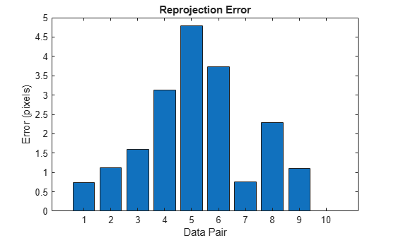
Based on the error metrics, you can choose to exclude some of the data pairs from the calibration to improve the accuracy of the results. For example, you can exclude the data pair with the largest reprojection error as follows.

Determine which data pair has the largest reprojection error.

[~,idxToExclude] = max(errors.ReprojectionError);

Remove the values of the data pair to exclude.

cornersCamera(:,:,idxToExclude) = NaN;
cornersLidar(:,:,idxToExclude) = NaN;

Repeat the calibration.

[lidarCameraTform,errors] = estimateLidarCameraTransform(ptCloudBoard,...
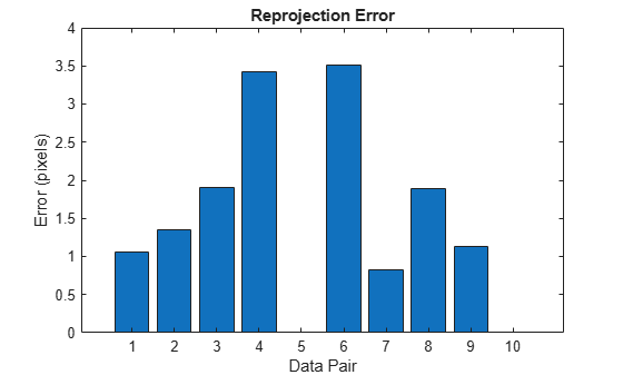
    cornersCamera,intrinsics,Lidar3DCorners=cornersLidar);

Plot the reprojection error after excluding the selected data pair.

figure
bar(errors.ReprojectionError)
title("Reprojection Error")
xlabel("Data Pair")
ylabel("Error (pixels)")

Fuse Lidar and Camera Data

After refining the lidar camera calibration results, you can use the transformation between the sensors to add color information to the point cloud. This section of the example uses the MultiSensorDrivingData_Seg7_Seq30 data which includes lidar and camera data collected with the same sensor setup used for calibration in the previous sections. Note that the dataset is approximately 1.8 GB.

Use the helperDownloadDataset supporting function to download the data as a struct.

if ~exist('recordedData','var')
    recordedData = helperDownloadDataset();
end

Lidar camera calibration results in a transformation that aligns the lidar frame to the camera frame. To add color information to the point cloud, you need the inverse of this transformation which is the transformation that aligns the camera frame to the lidar frame.

cameraLidarTform = invert(lidarCameraTform);

Now, for each available data pair, repeat the following steps:

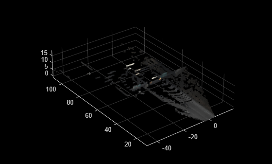
1) Get the point cloud frame.

numFrame = 1;
ptCloud = recordedData.Lidar.PointClouds{numFrame};
figure
pcshow(ptCloud)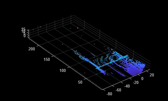

2) Find which image corresponds to the point cloud using the timestamps.

cameraTimestamps = recordedData.Camera.Timestamps;
ptCloudTimestamp = recordedData.Lidar.Timestamps(numFrame);
[~,idxImage] = min(abs(cameraTimestamps - ptCloudTimestamp));

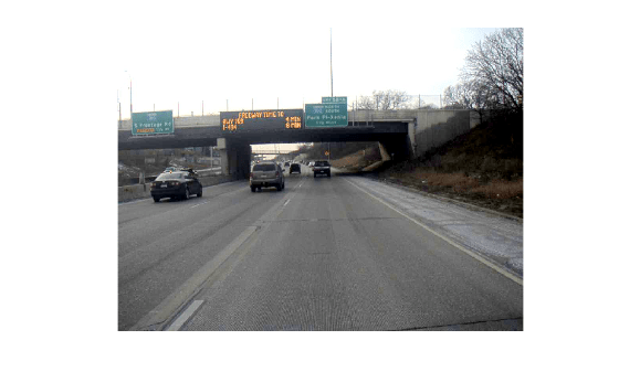
3) Get the corresponding image frame.

I = recordedData.Camera.Images{idxImage};
figure
imshow(I)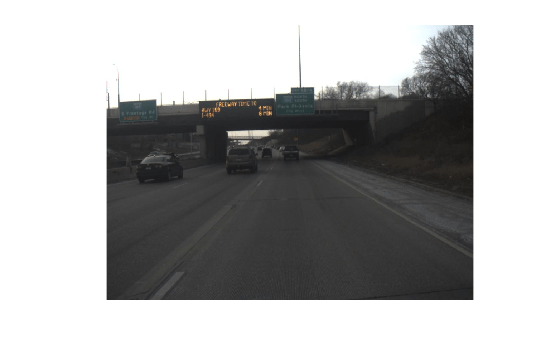

4) Enhance the brightness of the image using the imlocalbrighten function.

Ienhanced = imlocalbrighten(I);
figure
imshow(Ienhanced)

5) Add color information to the point cloud using the fuseCameraToLidar function.

ptCloudColor = fuseCameraToLidar(I,ptCloud,intrinsics,cameraLidarTform);
figure
pcshow(ptCloudColor,MarkerSize=20)
ylim([10 110])

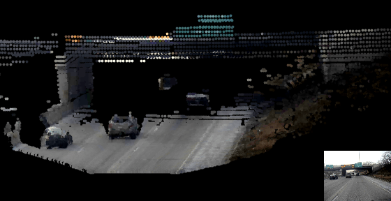
Now repeat steps 1-5 for the rest of the frames. To visualize the results, you can use pcplayer and add an axes on the bottom right corner to simultaneously visualize the image.

Set up pcplayer for point cloud visualization.

% Close existing plots and clear player from previous runs.
close all
if exist("player","var")
    clear player
end
figure(WindowState="maximized")
axPtCloud = axes;
player = pcplayer([-60 60],[0 150],[-5 30],Parent=axPtCloud,MarkerSize=75,AxesVisibility="off");

Modify the camera position and view to improve the visualization.

axPtCloud.CameraPosition = [12 -105 5];
axPtCloud.CameraTarget = [-2 88 2];
axPtCloud.CameraUpVector = [0 0 1];
axPtCloud.CameraViewAngle = 5;

Create an inset axes to visualize the image.

axImage = axes('Position',[0.79 0 0.25 0.25]);
box on;

Repeat steps 1-5 for all point clouds.

numPtClouds = numel(recordedData.Lidar.PointClouds);

for i = 1:numPtClouds
    % Get point cloud and its corresponding timestamp
    ptCloud = recordedData.Lidar.PointClouds{i};
    ptCloudTimestamp = recordedData.Lidar.Timestamps(i);
    
    % Find the image that corresponds to the point cloud based on
    % timestamps
    [~,index] = min(abs(cameraTimestamps - ptCloudTimestamp));
    I = recordedData.Camera.Images{index};
    
    % Enhance the color of the image
    I = imlocalbrighten(I);
    
    % Display the image
    imshow(I,Parent=axImage)
    
    % Add color information to the point cloud
    ptCloudColor = fuseCameraToLidar(I,ptCloud,intrinsics,cameraLidarTform);
    
    % Display the point cloud
    view(player,ptCloudColor);
end

close(axPtCloud.Parent)

References

[1] Zhou, Lipu, Zimo Li, and Michael Kaess. “Automatic Extrinsic Calibration of a Camera and a 3D LiDAR Using Line and Plane Correspondences.” In 2018 IEEE/RSJ International Conference on Intelligent Robots and Systems (IROS), 5562–69. Madrid: IEEE, 2018. https://doi.org/10.1109/IROS.2018.8593660.

[2] Arun, K. S., T. S. Huang, and S. D. Blostein. “Least-Squares Fitting of Two 3-D Point Sets.” IEEE Transactions on Pattern Analysis and Machine Intelligence PAMI-9, no. 5 (September 1987): 698–700. https://doi.org/10.1109/TPAMI.1987.4767965.