Results for
In a previous discussion,
we looked at a variety of infallible tests for primality, but all of them were too slow to be viable for large numbers. In fact, all of the methods discussed there will fail miserably for even moderately large numbers, those with just a few dozen decimal digits. That does not even begin to push into the realm of large numbers. In turn, that forces us into a different realm of tests - tests which are usually and even almost always correct, but can sometimes incorrectly predict primality.
In this discussion, I will be trying to convince you that the Fermat test for primality can be a quite good test when the number is sufficiently large. Except of course, when it is really bad. Even so, the Fermat test for primality is both a useful tool as well as a necessary underpinning for several other better tests.
The Fermat test for primality relies on Fermat's little theorem, a perhaps under-appreciated tool. Even the name implies it is of little interest. I'm not taking about the famous last theorem, only proven in recent years, but his little theorem.
If you want to look over some nice ways to prove the little theorem, take a read in this link:
I will readily admit that long ago, when I learned about the little theorem in a nearly forgotten class, I thought it was interesting, but why would I care? Not until I learned more mathematics and saw Fermat’s little theorem appearing in different places did I begin to appreciate it. Fermat tells us that, IF P is a prime, AND w is co-prime with P (so the two are relatively prime, sharing no common factors except 1), then it must be true that
mod(w^(P-1),P) == 1
Try it out. Does it work? Be careful though as too large of an exponent will cause problems in double precision, and that is not difficult to do. As a test case that will not overwhelm doubles, note that 13 is prime, and 3 shares no common factors with 13, so we satisfy the requirements for Fermat's little theorem.
mod(3^12,13)
We can even verify that any co-prime of 13 will yield the same result.
mod((1:12).^12,13)
Indeed it worked, suggesting what we knew all along, that 13 is prime. The little Fermat test for primality of the number P uses a converse form of Fermat's little theorem, thus given a co-prime number w known as the witness, is that if
mod(w^(P-1),P)==1
then we have evidence that P is indeed prime. This is not conclusive evidence, but still it is evidence. It is not conclusive because the converse of a true statement is not always true.
The analogy I like here is if we lived in a universe where all crows are black. (I'll ask you to pretend this is true. In fact, some crows have a mutation, making them essentially albino crows. For the purposes of this thought experiment, pretend this cannot happen.) Now, suppose I show you a picture of a bird which happens to be black. Do you know the bird to be a crow? Of course not, as the bird may be a raven, or a redwing blackbird (until you see the splash of red on the wing), a common grackle, a European starling in summer plumage, a condor, etc. But having seen black plumage, it is now more likely the bird is indeed a crow. I would call this a moderately weak evidentiary test for crow-ness.
Little Fermat may seem to be of little value when testing for primality for two reasons. First, computing the remainder would seem to be highly CPU intensive for large P. In the example above, I had only to compute 3^12=531441, which is not that large. But for numbers with many thousands or millions of digits, directly raising even a number as small as 2 to that power will overwhelm any computer. Secondly, if we do that computation, little Fermat does not conclusively prove P to be prime.
Our savior in one respect is the powermod tool. And that helps greatly, since we can compute the remainder in a reasonable time. A powermod call is quite fast even for huge powers. (I won't get into how powermod works here, since that alone is probably worth a discussion. I could though, if I see some interest because there are some very pretty variations of the powermod algorithm. I hope to show you one of them when I discuss the Fibonacci test for primality in a future post.) Trying the little Fermat test using powermod on a number with 1207 decimal digits, I’ll first do a time check.
P = 4000*sym(2)^3999 - 1;
timeit(@() powermod(2,P-1,P))
As you can see, powermod really is pretty fast. Compared to an isprime test on that number it would show a significant difference.
I have said before that little Fermat is not a conclusive test. In fact, a good trick is to perform a second little Fermat test, using a different witness. If the second test also indicates primality, then we have additional evidence that P is in fact prime.
w = [2 3]; % Two parallel witnesses
powermod(w,P-1,P)
This value for P is indeed prime, and little Fermat suggests it is, doubly suggestive in that test since I actually performed two parallel tests. Here however, we need to understand when it will fail, and how often it will fail.
If we perform a little Fermat test for primality, we will never see false negatives, that is, if any test with any witness ever indicates a number is composite, then it is certainly composite. (The contrapositive of a true statement is always true.) The alternate class of failure is the false positive, where little Fermat indicates a number is prime when it was actually composite.
If P is composite, and w co-prime with P, we call P a Fermat pseudo-prime for the witness w if we see a remainder of 1 when P was in fact composite. When that happens, the witness (w) is called a Fermat liar for the primality of P. (A list of some Fermat pseudo-primes where 2 is a Fermat liar can be found in sequence A001567 of the OEIS.)
In the case of 4000*2^3999-1, I claimed the number to be in fact prime, and it was identified so (as PROBABLY prime by little Fermat. Next, consider another number from that same family. I’ll perform three parallel tests on it, with witnesses 2, 3, and 5. This will suggest the value of doing parallel tests on a number to reduce the failure rate from little Fermat.
P2 = 1024*sym(2)^1023 - 1;
w = [2; 3; 5];
gcd(w,P2)
F2 = powermod(w,P2-1,P2)
logical(F2 == 1)
As you can see, P2 is co-prime with all of 2, 3 and 5, but 2 is a Fermat liar, whilst 3 and 5 are Fermat truth tellers, identifying P2 as certainly composite. So the little Fermat test can definitely fail for SOME witnesses, since we see a disagreement. However, an interesting fact about P2 above is it is also a Mersenne number with prime exponent, thus it can be written as 2^1033-1, where 1033 is prime. I can go into more detail about this case later, but we can show that 2 is always a Fermat liar for composite Mersenne numbers when the exponent is itself prime. I’ll try to leave more detail on this matter in a future discussion, or perhaps a comment.
Next, consider the composite integer 51=3*17. As the product of two primes, it is clearly not itself prime.
P51 = 51;
w0 = 2:P51-2;
w = w0(gcd(w0,P51) == 1)
Note that I did not include 1 or 50 in that set, since 1 raised to any power is 1, and 50 is congruent to -1, mod 51. -1 raised to any even power is also always 1, and 51-1 is an even number. And so when we are working modulo 51, both 1 and 50 are not useful witnesses in terms of the little Fermat test.
R = powermod(w,P-1,P)
w(R == 1)
This teaches us that when 51 is tested for primality using the little Fermat test, there are 2 distinct witnesses w (16 and 35) we could have chosen which would have been Fermat liars, but all 28 other potential co-prime witnesses would have been truth tellers, accurately showing 51 to be composite. Proportionally, little Fermat will have been correct roughly 93% of the time, since only 2 of these 30 possible tests returned a false positive. (I’ll add that for any modulus P, if w<P is not co-prime with the modulus, then the computation mod(w^(P-1),P) will always return a non-unit result, and therefore we can theoretically use any integer w from the set 2:P-2 as a witness. However if w is co-prime with P then P is clearly not prime, and the entire problem becomes a little less interesting. As such, I will only consider co-prime witnesses for this discussion.) Regardless, that would make the little Fermat test for P=51 even more often correct, since it returns the correct result of composite for 46 out of the 48 possible witnesses 2:49. Does this mean Little Fermat is indeed the basis for a good test to rely on to learn if a number is prime? Well, yes. And no.
Little Fermat forms a very good test most of the time, but reliance is a strong word. This means we need to explore the little Fermat test in more depth, focusing on Fermat liars and the case of false positives. To offer some appreciation of the false positive rate, offline, I have tested all composite integers between 4 and 10000, for all their possible co-prime witnesses.
load FermatLiarsData
In that .mat file, I've saved three vectors, X, witnessCount, and liarCount. X is there just to use for plotting purposes and is NaN for all non-composite entries.
whos X witnessCount liarCount
The vector witnessCount is the number of valid witnesses for the corresponding number in X. Corresponding to that is the vector liarCount, which is the number of Fermat liars I found for each composite in X.
How many Fermat test useful witnesses are there for any integer X? This is just 2 less than the number of coprimes of X. The number of coprimes is given by the Euler totient function, commonly called phi(X). (I’ll be going into more depth on the totient in the next chapter of this series, because the Euler totient is a crucial part of understanding how all of this works.)
The witness count is phi(X)-2. Why subtract 2? 1 can never be a witness, but 1 is technically coprime to everything. The same applies to X-1 (which is congruent to -1 mod X.) As such, there are phi(X)-2 coprimes to consider. (I've posted a function called totient on the FEX, but it is easily computed if you know the factorization of X. Or for small numbers, you can just use GCD to identify all co-primes, and count them.)
plot(X,witnessCount,'.')
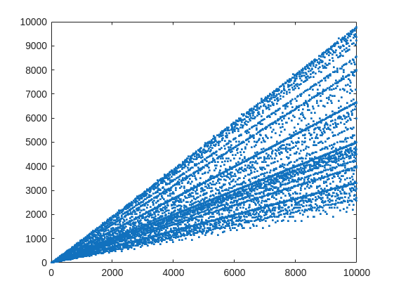
From that plot, you can learn a few interesting things. (As a mathematician, this is what I love the most, thus to look at whay may be the simplest, most boring plot, and try to find something of value, something I had never thought of before.) For example, we know that when X is prime, then everything from the set 2:X-2 is a valid witness. So the upper boundary on that plot will be the line y==x. As well, there are a few numbers where the order of the set of witnesses will be close to the maximum possible. For example, 961=31*31, has 928 valid witnesses. That makes some sense, as 961 is the square of a prime (31), so we know 961 is divisible only by 31. Only multiples of 31 will not be coprime with 961.
But how about the lower boundary? The least number of valid witnesses will always come from highly composite numbers, because they will share common factors with almost everything. For example 30 = 2*3*5, or 210=2*3*5*7.
witnessCount([30 210 420])
A good discussion about the lower bound for that plot can be found here:
What really matters to us though, is the fraction of the useful witnesses for a little Fermat test that yield a false positive.
plot(X,liarCount./witnessCount,'b.')
Cind = liarCount == witnessCount;
hold on
plot(X(Cind),1,'ro')
ylabel('Liar fraction')
xlabel('X')
title('Fermat pseudo-prime strength')
hold off
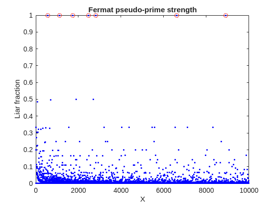
A look at this plot shows seven circles in red, corresponding to X from the list {561, 1105, 1729, 2465, 2821, 6601, 8911} which are collectively known as Carmichael numbers. These are numbers where all witnesses return a false positive. Carmichael numbers are themselves fairly rare. You can find a list of them as sequence A002997 in the OEIS. And for those of you who have never wandered around the OEIS, please take this opportunity to do so now. The OEIS stands for Online Encyclopedia of Integer Sequences. It contains a wealth of interesting knowledge about integers and integer sequences.)
There are a few other interesting numbers we can find in that plot, like 91 and 703, where roughly 50% of the valid witnesses yield false positives. Of the complete set, which numbers did return at least a 25% false positive rate for primality? These numbers would be known as strong pseudo-primes for the little Fermat test, because they are pseudo-primes for at least 25% of the potential witnesses. These strong pseudo-primes have some interesting similarities to the Carmichael numbers. (My next post will go into more depth on Carmichael numbers and strong pseudo-primes. At the moment, I am merely interested in looking at the how often the little Fermat test fails overall.)
find(liarCount./witnessCount> 0.25)
You should notice the spacing between successive strong Fermat pseudo-primes is growing slowly, with a spacing of roughly 800 on average in the vicinity of 10000. If I step out beyond by a factor of 10, the next strong Fermat pseudo-primes after 1e5 are {101101, 104653, 107185, 109061, 111361, 114589, 115921 126217, 126673}, so that average spacing is definitely growing.
Given that set, now we can look at the prime factorizations of each of those strong pseudo-primes. Can we learn something about them?
arrayfun(@factor,find(liarCount./witnessCount> 0.25),'UniformOutput',false)
Perhaps the most glaring thing I see in that set of factors is almost all of those strong Fermat pseudo-primes are square free. That is, in that list, only 45=3*3*5 had any replicated factor at all. That property of being square free is something we will see is necessary to be a Carmichael number, but it also suggests that a simple roughness test applied in advance would have eliminated almost all of those strong pseudo-primes as obviously not prime, even at a very low level of roughness.
In fact, for most composite integers, most witnesses do indeed return a negative, indicating the number is not prime, and therefore composite. Little Fermat does not commonly tell falsehoods, even though it can do so.
semilogy(X,movmedian(liarCount./witnessCount,20,'omitnan'),'b-')
title('False positive fraction for composites')
yline(0.0003,'r')

We can learn from this last plot that as the number to be tested grows large, the median false positive rate for little Fermat, even for X as low as only 10000, is roughly 0.0003. (It continues to decrease for larger X too. In fact, I’ve read that when X is on the order of 2^256, the relative fraction of Fermat liars is on the order of 1 in 1e12, and it continues to decrease as X grows in magnitude. In my eyes, that seems pretty good for an imperfect test. Not perfect, but not bad when paired with roughness and perhaps a second little Fermat test using a different witness, and we will start to see tests which bear a higher degree of strength.)
I’ll stop at this point in this post because the post is getting lengthy. In my next post, I’d like to visit some questions about what are Carmichael numbers, about whether some witnesses are better than others, and if there are any numbers which lack any Fermat liars. However, in order to dive more deeply, I will need to explain how/why/when the little Fermat test works, and what causes Fermat liars. Stay tuned, because this starts to get interesting.
If you have published add-ons on File Exchange, you may have noticed that we recently added a new, unique package name field to all add-ons. This enables future support for automated installation with the MATLAB Package Manager. This name will be a unique identifier for your add-on and does not affect the existing add-on title, any file names, or the URL of your add-on.
📝 Update and review until April 10
We generated default package names for all add-ons. You can review and update the package name for your add-ons until April 10, 2026. Review your package names now:
After April 10, you will need to create a new version to change your package name.
🚀 More changes coming with the MATLAB R2026b prerelease
Starting with the MATLAB R2026b prerelease, these package names will take effect. At that time, the package name may appear on the File Exchange page for your add-on.
Keep your eyes peeled for exciting changes coming soon to your add-ons on File Exchange!
Cantera is an open-source suite of tools for problems involving chemical kinetics, thermodynamics, and transport processes. Dr. Su Sun, a recent graduate from Northeastern Chemical Engineering Ph.D. program made significant contributions to MATLAB interface for Cantera in Cantera Release 3.2.0 in collaboration with Dr. Richard West, other Cantera developers, and MathWorks Advanced Support and Development Teams. As part of this Release, MATLAB interface for Cantera transitioned to using the new MATLAB- C++ interface and expanded their unit testing. Further information is available here.
I began coding in MATLAB less than 2 months ago for a class at community college. Alongside the course content, I also completed the MATLAB onramp and introduction to linear algebra self-paced online courses. I think this is the most fun I've had coding since back when I used to make Scratch projects in elementary school. I'm kind of curious if I could recreate some of my favorite childhood Scratch games here.
Anyways, I just wanted to introduce myself since I plan to be really active this year. My name is Mehreen (meh like the meh emoji from the Emoji movie, reen like screen), I'm a data science undergrad sophomore from the U.S. and it's nice to meet you!
An emirp is a prime that is prime when viewed in in both directions. They are not too difficult to find at a lower level. For example...
isprime([199 991])
Gosh, that was easy. But what happens if the number is a bit larger? The problem is, primes themselves tend to be rare on the number line when you get into thousands or tens of thousands of decimal digits. And recently, I read that a world record size prime had been found in this form. You have probably all heard of Matt Parker and numberphile.
And so, I decided that MATLAB would be capable of doing better. Why not? After all, at the time, the record size emirp had only 10002 decimal digits.
How would I solve this problem? First, we can very simply write a potential emirp as
10^n + a
then we can form the flipped version as
ahat*10^(n-d) + 1
where ahat is the decimally flipped version of a, and d is chosen based on the number of decimal digits in the number a itself. Not all emirps will be of that form of course, but using all of those powers of 10 makes it easy to construct a large number and its reversed form. And that is a huge benefit in this. For example,
Pfor = sym(10)^101 + 943
Prev = 349*sym(10)^99 + 1
It is easier to view these numbers using a little code I wrote, one that redacts most of those boring zeros.
emirpdisplay(Pfor)
emirpdisplay(Prev)
And yes, they are both prime, and they both have 102 decimal digits.
isprime([Pfor,Prev])
Sadly, even numbers that large are very small potatoes, at least in the world of large primes. So how do we solve for a much larger prime pair using MATLAB?
The first thing I want to do is to employ roughness at a high level. If a number is prime, then it is maximally rough. (I posted a few discussions about roughness some time ago.)
https://www.mathworks.com/matlabcentral/discussions/tips/879745-primes-and-rough-numbers-basic-ideas
In this case, I'm going to look for serious roughness, thus 2e9-rough numbers. Again, a number is k-rough if its smallest prime factor is greater than k. There are roughly 98 million primes below 2e9.
The general idea is to compute the remainders of 10^12345, modulo every prime in that set of primes below 2e9. This MUST be done using int64 or uint64 arithmetic, as doubles will start to fail you above
format short g
sqrt(flintmax)
The sqrt is in there because we will be multiplying numbers together here, and we need always to stay below intmax for the integer format you are working with. However, if we work in an integer format, we can get as high as 2e9 easily enough, by going to int64 or uint64.
sqrt(double(intmax('int64')))
And, yes, this means I could have gone as high as primes(3e9), however, I stopped at 2e9 due to the amount of RAM on my computer. 98 million primes seemed enough for this task. And even then, I found myself working with all of the cores on my computer. (Note that I found int64 arithmetic will only fire up the performance cores on your Mac via automatic multi-threading. Mine has 12 performance cores, even though it has 16 total cores.)
I computed the remainders of 10^12345 with respect to each prime in that set using a variation of the powermod algorithm. (Not powermod itself, which was itself not sufficiently fast for my purposes.) Once I had those 98 millin remainders in a vector, then it became easy to use a variation of the sieve of Eratosthenes to identify 2e9-rough numbers.
For example, working at 101 decimal digits, if I search for primes of the form 10^101+a, with a in the interval [1,10000], there are 256 numbers of that form which are 2e9-rough. Roughness is a HUGE benefit, since as you can see here, I would not want to test for primality all 10000 possible integers from that interval.
Next, I flip those 256 rough numbers into their mirror image form. Which members of that set are also rough in the mirror image form? We would then see this further reduces the set to only 34 candidates we need test for primality which were rough in both directions. With now only a few direct tests for primality, we would find that pair of 102 digit primes shown above.
Of course, I'm still needing to work with primes in the regime of 10000 plus decimal digits, and that means I need to be smarter about how I test a number to be prime. The isprime test given by sym/isprime only survives out to around 1000 decimal digits before it starts to get too slow. That means I need to perform Fermat tests to screen numbers for primality. If that indicates potential primality, I currently use a Miller-Rabin code to verify that result, one based on the tool Java.Math.BigInteger.isProbablePrime.
And since Wikipedia tells me the current world record known emirp was
117,954,861 * 10^11111 + 1 discovered by Mykola Kamenyuk
that tells me I need to look further out yet. I chose an exponent of 12345, so starting at 10^12345. Last night I set my Mac to work, with all cores a-fumbling, a-rumbling at the task as I slept. Around 4 am this morning, it found this number:
emirp = @(N,a) sym(10)^N + a;
Pfor = emirp(12345,10519197);
Prev = sym(flip(char(Pfor)));
emirpdisplay(Pfor)
emirpdisplay(Prev)
isProbablePrimeFLT([Pfor,Prev],210)
I'm afraid you will need to take my word for it that both also satisfy a more robust test of primality, as even a Miller-Rabin test that will take more time than the MATLAB version we get for use in a discussion will allow. As far as a better test in the form of the MATLAB isprime utility to verify true primality, that test is still running on my computer. I'll check back in a few hours to see if it fininshed.
Anyway, the above numbers now form the new world record known emirp pair, at 12346 decimal digits. Yes, I do recognize this is still what I would call low hanging fruit, that having announced a largest prime of this form, someone else willl find one yet larger in a few weeks or months. But even so, for the moment, MATLAB owns the world record!
If anyone else wants a version of the codes I used for the search, I've attached a version (emirpsearchpar.m) that employs the parallel processing toolbox. I do have as well a serial version which is of course, much, much slower. It would be fun to crowd source a larger world record yet from the MATLAB community.
Hey folks in MATLAB community! I'm an engineering student from India messing around with deep learning/ML for spotting faults in power electronics stuff—like inverter issues or microgrid glitches in Simulink.
What's your take?
- Which toolbox rocks for this—Deep Learning one or Predictive Maintenance?
- Any gotchas when training on sim data vs real hardware?
- Cool workflows or GitHub links you've used?
Would love your real experiences! 😊
The "Issues" with Constant Properties
MATLABs Constant properties can be rather difficult to deal with at times. For those unfamiliar there are two distinct behaviors when accessing constant properties of a class. If a "static" pattern is used ClassName.PropName the the value, as it was assigned to the property is returned; that is to say that you will have a nargout of 1. But, rather frustratingly, if an instance of the class is used when accessing the constant property, such as ArrayOfClassName.PropName then your nargout will be equivalent to the number of elements in the array; this means that functionally the constant property accessing scheme is identical to that of the element wise properties you find on "instance" properties.
Motivation for Correcting Constant Property Behavior
This can be frustraing since constant properties are conceptually designed to tie data to a class. You could see this design pattern being useful where a super class were to define an abstract constant property, that would drive the behavior of subclasses; the subclasses define the value of the property and the super class uses it. I would like to use this design to develop a custom display "MatrixDisplay" focused mixin (like the internal matlab.mixin.internal.MatrixDisplay). The idea is that missing element labels, invalid handle element labels, and other semantic values can be configured by the subclasses, conveniently just by setting the constant properties; these properties will be used by the super class to substitute the display strings of appropriate elements. Most of the processing will happen within the super class as to enable simple, low-investment, opt-in display options for array style classes.
The issue is that you can not rely on constant property access to return the appropriate value when the instance you've been passed is empty. This also happens with excessive outputs when the instance is non-scalar, but those extra values from the CSL are just ignored, while Id imagine there is an effect on performance from generating the excess outputs (assuming theres no internal optimization for the unused outputs), this case still functions appropriately. As I enjoying exploring MATLAB, I found an internal indexing mixing class in the past that provides far greater control of do indexing; I've done a good deal of neat things with it, though at the cost of great overhead when getting implementing cool "proof of concept/showcase" examples. Today I used it to quickly implement a mix in that "fixes" constant properties such that they always return as though they were called statically from the class name, as opposed to an instance.
A Simplistic Solution
To do this I just intercepted the property indexing, checked if it was constant, and used the DefaultValue property of the metadata to return the value. This works nicely since we are required to attempt to initialize a "dummy" scalar array, or generate a function handle; both of those would likely be slower, and in the former case, may not be possible depending on the subclass implementation. It is worth noting that this method of querying the value from metadata is safe because constant properties are immutable and thus must be established as the class is loaded. Below is the small utility class I have implemented to get predictable constant variable access into classes that benefit from it. Lastly it is worth noting that I've not torture testing the rerouting of the indexing we aren't intercepting, in my limited play its behaved as expected but it may be worth looking over if you end up playing around with this and notice abnormal property assignment or reading from non-constant properties.
Sample Class Implementation
classdef(Abstract, HandleCompatible) ConstantProperty < matlab.mixin.internal.indexing.RedefinesDotProperties
%ConstantProperty Returns instance indexed constant properties as though they were statically indexed.
% This class overloads property access to check if the indexed property is constant and return it properly.
%% Property membership utility methods
methods(Access=private)
function [isConst, isProp] = isConstantProp(obj, prop, options)
%isConstantProp Determine if the input property names are constant properties of the input
arguments
obj mixin.ConstantProperty;
prop string;
options.Flatten (1, 1) logical = false;
end
% Store the cache to avoid rechecking string membership and parsing metadata
persistent class_cache
% Initialize cache for all subclasses to maintain their own caches
if(isempty(class_cache))
class_cache = configureDictionary("string", "dictionary");
end
% Gather the current class being analyzed
classname = string(class(obj));
% Check if the current class has a cache, if not make one
if(~isKey(class_cache, classname))
class_cache(classname) = configureDictionary("string", "struct");
end
% Alias the current classes cache
prop_cache = class_cache(classname);
% Check which inputs are already cached
isCached = isKey(prop_cache, prop);
% Add any values that have yet to be cached to the cache
if(any(~isCached, "all"))
% Flatten cache additions
props = row(prop(~isCached));
% Gather the meta-property data of the input object and determine if inputs are listed properties
mc_props = metaclass(obj).PropertyList;
% Determine which properties are keys
[isConst, idx] = ismember(props, string({mc_props.Name}));
idx = idx(isConst);
% Check which of the inputs are constant properties
isConst = repmat(isConst, 2, 1);
isConst(1, isConst(1, :)) = [mc_props(idx).Constant];
% Parse the results into structs for caching
cache_values = cell2struct(num2cell(isConst), ["isConst"; "isProp"]);
prop_cache(props) = row(cache_values);
% Re-sync the cache
class_cache(classname) = prop_cache;
end
% Extract results from the cache
values = prop_cache(prop);
if(options.Flatten)
% Split and reshape output data
sz = size(prop);
isConst = reshape(values.isConst, sz);
isProp = reshape(values.isProp, sz);
else
isConst = struct2cell(values);
end
end
function [isConst, isProp] = isConstantIdxOp(obj, idxOp)
%isConstantIdxOp Determines if the idxOp is referencing a constant property.
arguments
obj mixin.ConstantProperty;
idxOp (1, :) matlab.indexing.IndexingOperation;
end
import matlab.indexing.IndexingOperationType;
if(idxOp(1).Type == IndexingOperationType.Dot)
[isConst, isProp] = isConstantProp(obj, idxOp(1).Name);
else
[isConst, isProp] = deal(false);
end
end
function A = getConstantProperty(obj, idxOp)
%getConstantProperty Returns the value of a constant property using a static reference pattern.
arguments
obj mixin.ConstantProperty;
idxOp (1, :) matlab.indexing.IndexingOperation;
end
A = findobj(metaclass(obj).PropertyList, "Name", idxOp(1).Name).DefaultValue;
end
end
%% Dot indexing methods
methods(Access = protected)
function A = dotReference(obj, idxOp)
arguments(Input)
obj mixin.ConstantProperty;
idxOp (1, :) matlab.indexing.IndexingOperation;
end
arguments(Output, Repeating)
A
end
% Force at least one output
N = max(1, nargout);
% Check if the indexing operation is a property, and if that property is constant
[isConst, isProp] = isConstantIdxOp(obj, idxOp);
if(~isProp)
% Error on invalid properties
throw(MException( ...
"JB:mixin:ConstantProperty:UnrecognizedProperty", ...
"Unrecognized property '%s'.", ...
idxOp(1).Name ...
));
elseif(isConst)
% Handle forwarding indexing operations
if(isscalar(idxOp))
% Direct assignment
[A{1:N}] = getConstantProperty(obj, idxOp);
else
% First extract constant property then forward indexing operations
tmp = getConstantProperty(obj, idxOp);
[A{1:N}] = tmp.(idxOp(2:end));
end
else
% Handle forwarding indexing operations
if(isscalar(idxOp))
% Unfortunately we can't just recall obj.(idxOp) to use default/built-in so we manually extract
[A{1:N}] = obj.(idxOp.Name);
else
% Otherwise let built-in handling proceed
tmp = obj.(idxOp(1).Name);
[A{1:N}] = tmp.(idxOp(2:end));
end
end
end
function obj = dotAssign(obj, idxOp, values)
arguments(Input)
obj mixin.ConstantProperty;
idxOp (1, :) matlab.indexing.IndexingOperation;
end
arguments(Input, Repeating)
values
end
% Handle assignment based on presence of forward indexing
if(isscalar(idxOp))
% Simple broadcasted assignment
[obj.(idxOp.Name)] = deal(values{:});
else
% Initialize the intermediate values and expand the values for assignment
tmp = {obj.(idxOp(1).Name)};
[tmp.(idxOp(2:end))] = deal(values{:});
% Reassign the modified data to the output object
[obj.(idxOp(1).Name)] = deal(tmp{:});
end
end
function n = dotListLength(obj, idxOp, idxCnt)
arguments(Input)
obj mixin.ConstantProperty;
idxOp (1, :) matlab.indexing.IndexingOperation;
idxCnt (1, :) matlab.indexing.IndexingContext;
end
if(isConstantIdxOp(obj, idxOp))
if(isscalar(idxOp))
% Constant properties will also be 1
n = 1;
else
% Checking forwarded indexing operations on the scalar constant property
n = listLength(obj.(idxOp(1).Name), idxOp(2:end), idxCnt);
end
else
% Check the indexing operation normally
% n = listLength(obj, idxOp, idxCnt);
n = numel(obj);
end
end
end
end
k-Wave is a MATLAB community toolbox with a track record that includes over 2,500 citations on Google Scholar and over 7,500 downloads on File Exchange. It is built for the "time-domain simulation of acoustic wave fields" and was recently highlighted as a Pick of the Week.
In December, release v1.4.1 was published on GitHub including two new features led by the project's core contributors with domain experts in this field. This first release in several years also included quality and maintainability enhancements supported by a new code contributor, GitHub user stellaprins, who is a Research Software Engineer at University College London. Her contributions in 2025 spanned several software engineering aspects, including the addition of continuous integration (CI), fixing several bugs, and updating date/time handling to use datetime. The MATLAB Community Toolbox Program sponsored these contributions, and welcomes to see them now integrated into a release for k-Wave users.
I'd like to share some work from Controls Educator and long term collabortor @Dr James E. Pickering from Harper Adams University. He is currently developing a teaching architecture for control engineering (ACE-CORE) and is looking for feedback from the engineering community.
ACE-CORE is delivered through ACE-Box, a modular hardware platform (Base + Sense, Actuate). More on the hardware here: What is the ACE-Box?
The Structure
(1) Comprehend
Learners build conceptual understanding of control systems by mapping block diagrams directly to physical components and signals. The emphasis is on:
- Feedback architecture
- Sensing and actuation
- Closed-loop behaviour in practical terms
(2) Operate
Using ACE-Box (initially Base + Sense), learners run real closed-loop systems. The learners measure, actuate, and observe real phenomena such as: Noise, Delay, Saturation
Engineering requirements (settling time, overshoot, steady-state error, etc.) are introduced explicitly at this stage.
After completing core activities (e.g., low-pass filter implementation or PID tuning), the pathway branches (see the attached diagram)
(3a) Refine (Option 1) Students improve performance through structured tuning:
- PID gains
- Filter coefficients
- Performance trade-offs
The focus is optimisation against defined engineering requirements.
(3b) Refine → Engineer (Option 2)
Modelling and analytical design become more explicit at this stage, including:
- Mathematical modelling
- Transfer functions
- System identification
- Stability analysis
- Analytical controller design
Why the Branching?
The structure reflects two realities:
- Engineers who operate and refine existing control systems
- Engineers who design control systems through mathematical modelling
Your perspective would be very valuable:
- Does this progression reflect industry reality?
- Is the branching structure meaningful?
- What blind spots do you see?
Constructive critique is very welcome. Thank you!
Hello All,
This is my first post here so I hope its in the right place,
I have built myself a GW consisting of a RAK2245 concentrator and a Raspberry Pi, Also an Arduino end device from this link https://tum-gis-sensor-nodes.readthedocs.io/en/latest/dragino_lora_arduino_shield/README.html
Both projects work fine and connect to TTN whereby packets of data from the end device can be seen in the TTN console.
I now want to create a Webhook in TTN for Thingspeak which would hopefull allow me to see Temperature , Humidity etc in graphical form.
My question, does thingspeak support homebuilt devices or is it focused on comercially built devices ?
I have spent many hours trying to find data hosting site that is comepletely free for a few devices and not to complicated to setup as some seem to be a nightmare. Thanks for any support .
How can I found my license I'd and password, so please provide me my id
Over the past few days I noticed a minor change on the MATLAB File Exchange:
For a FEX repository, if you click the 'Files' tab you now get a file-tree–style online manager layout with an 'Open in new tab' hyperlink near the top-left. This is very useful:
If you want to share that specific page externally (e.g., on GitHub), you can simply copy that hyperlink. For .mlx files it provides a perfect preview. I'd love to hear your thoughts.
EXAMPLE:
🤗🤗🤗
I wanted to share something I've been thinking about to get your reactions. We all know that most MATLAB users are engineers and scientists, using MATLAB to do engineering and science. Of course, some users are professional software developers who build professional software with MATLAB - either MATLAB-based tools for engineers and scientists, or production software with MATLAB Coder, MATLAB Compiler, or MATLAB Web App Server.
I've spent years puzzling about the very large grey area in between - engineers and scientists who build useful-enough stuff in MATLAB that they want their code to work tomorrow, on somebody else's machine, or maybe for a large number of users. My colleagues and I have taken to calling them "Reluctant Developers". I say "them", but I am 1,000% a reluctant developer.
I first hit this problem while working on my Mech Eng Ph.D. in the late 90s. I built some elaborate MATLAB-based tools to run experiments and analysis in our lab. Several of us relied on them day in and day out. I don't think I was out in the real world for more than a month before my advisor pinged me because my software stopped working. And so began a career of building amazing, useful, and wildly unreliable tools for other MATLAB users.
About a decade ago I noticed that people kept trying to nudge me along - "you should really write tests", "why aren't you using source control". I ignored them. These are things software developers do, and I'm an engineer.
I think it finally clicked for me when I listened to a talk at a MATLAB Expo around 2017. An aerospace engineer gave a talk on how his team had adopted git-based workflows for developing flight control algorithms. An attendee asked "how do you have time to do engineering with all this extra time spent using software development tools like git"? The response was something to the effect of "oh, we actually have more time to do engineering. We've eliminated all of the waste from our unamanaged processes, like multiple people making similar updates or losing track of the best version of an algorithm." I still didn't adopt better practices, but at least I started to get a sense of why I might.
Fast-forward to today. I know lots of users who've picked up software dev tools like they are no big deal, but I know lots more who are still holding onto their ad-hoc workflows as long as they can. I'm on a bit of a campaign to try to change this. I'd like to help MATLAB users recognize when they have problems that are best solved by borrowing tools from our software developer friends, and then give a gentle onramp to using these tools with MATLAB.
I recently published this guide as a start:
Waddya think? Does the idea of Reluctant Developer resonate with you? If you take some time to read the guide, I'd love comments here or give suggestions by creating Issues on the guide on GitHub (there I go, sneaking in some software dev stuff ...)
I recently created a short 5-minute video covering 10 tips for students learning MATLAB. I hope this helps!
DocMaker allows you to create MATLAB toolbox documentation from Markdown documents and MATLAB scripts.
The MathWorks Consulting group have been using it for a while now, and so David Sampson, the director of Application Engineering, felt that it was time to share it with the MATLAB and Simulink community.
David listed its features as:
➡️ write documentation in Markdown not HTML
🏃 run MATLAB code and insert textual and graphical output
📜 no more hand writing XML index files
🕸️ generate documentation for any release from R2021a onwards
💻 view and edit documentation in MATLAB, VS Code, GitHub, GitLab, ...
🎉 automate toolbox documentation generation using MATLAB build tool
📃 fully documented using itself
😎 supports light, dark, and responsive modes
🐣 cute logo
I got an email message that says all the files I've uploaded to the File Exchange will be given unique names. Are these new names being applied to my files automatically? If so, do I need to download them to get versions with the new name so that if I update them they'll have the new name instead of the name I'm using now?
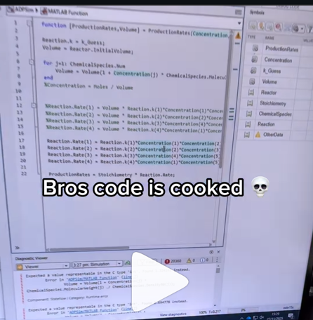
A coworker shared with me a hilarious Instagram post today. A brave bro posted a short video showing his MATLAB code… casually throwing 49,000 errors!
Surprisingly, the video went virial and recieved 250,000+ likes and 800+ comments. You really never know what the Instagram algorithm is thinking, but apparently “my code is absolutely cooked” is a universal developer experience 😂
Last note: Can someone please help this Bro fix his code?
Is it possible to display a variable value within the ThingSpeak plot area?
https://www.mathworks.com/matlabcentral/answers/2182045-why-can-t-i-renew-or-purchase-add-ons-for-m…
"As of January 1, 2026, Perpetual Student and Home offerings have been sunset and replaced with new Annual Subscription Student and Home offerings."
So, Perpetual licenses for Student and Home versions are no more. Also, the ability for Student and Home to license just MATLAB by itself has been removed.
The new offering for Students is $US119 per year with no possibility of renewing through a Software Maintenance Service type offering. That $US119 covers the Student Suite of MATLAB and Simulink and 11 other toolboxes. Before, the perpetual license was $US99... and was a perpetual license, so if (for example) you bought it in second year you could use it in third and fourth year for no additional cost. $US99 once, or $US99 + $US35*2 = $US169 (if you took SMS for 2 years) has now been replaced by $US119 * 3 = $US357 (assuming 3 years use.)
The new offering for Home is $US165 per year for the Suite (MATLAB + 12 common toolboxes.) This is a less expensive than the previous $US150 + $US49 per toolbox if you had a use for those toolboxes . Except the previous price was a perpetual license. It seems to me to be more likely that Home users would have a use for the license for extended periods, compared to the Student license (Student licenses were perpetual licenses but were only valid while you were enrolled in degree granting instituations.)
Unfortunately, I do not presently recall the (former) price for SMS for the Home license. It might be the case that by the time you added up SMS for base MATLAB and the 12 toolboxes, that you were pretty much approaching $US165 per year anyhow... if you needed those toolboxes and were willing to pay for SMS.
But any way you look at it, the price for the Student version has effectively gone way up. I think this is a bad move, that will discourage students from purchasing MATLAB in any given year, unless they need it for courses. No (well, not much) more students buying MATLAB with the intent to explore it, knowing that it would still be available to them when it came time for their courses.
You may have come across code that looks like that in some languages:
stubFor(get(urlPathEqualTo("/quotes"))
.withHeader("Accept", equalTo("application/json"))
.withQueryParam("s", equalTo(monitoredStock))
.willReturn(aResponse())
.withStatus(200)
.withHeader("Content-Type", "application/json")
.withBody("{\\"symbol\\": \\"XYZ\\", \\"bid\\": 20.2, " + "\\"ask\\": 20.6}")))
That’s Java. Even if you can’t fully decipher it, you can get a rough idea of what it is supposed to do, build a rather complex API query.
Or you may be familiar with the following similar and frequent syntax in Python:
import seaborn as sns
sns.load_dataset('tips').sample(10, random_state=42).groupby('day').mean()
Here’s is how it works: multiple method calls are linked together in a single statement, spanning over one or several lines, usually because each method returns the same object or another object that supports further calls.
That technique is called method chaining and is popular in Object-Oriented Programming.
A few years ago, I looked for a way to write code like that in MATLAB too. And the answer is that it can be done in MATLAB as well, whevener you write your own class!
Implementing a method that can be chained is simply a matter of writing a method that returns the object itself.
In this article, I would like to show how to do it and what we can gain from such a syntax.
Example
A few years ago, I first sought how to implement that technique for a simulation launcher that had lots of parameters (far too many):
lauchSimulation(2014:2020, true, 'template', 'TmplProd', 'Priority', '+1', 'Memory', '+6000')
As you can see, that function takes 2 required inputs, and 3 named parameters (whose names aren’t even consistent, with ‘Priority’ and ‘Memory’ starting with an uppercase letter when ‘template’ doesn’t).
(The original function had many more parameters that I omit for the sake of brevity. You may also know of such functions in your own code that take a dozen parameters which you can remember the exact order.)
I thought it would be nice to replace that with:
SimulationLauncher() ...
.onYears(2014:2020) ...
.onDistributedCluster() ... % = equivalent of the previous "true"
.withTemplate('TmplProd') ...
.withPriority('+1') ...
.withReservedMemory('+6000') ...
.launch();
The first 6 lines create an object of class SimulationLauncher, calls several methods on that object to set the parameters, and lastly the method launch() is called, when all desired parameters have been set.
To make it cleared, the syntax previously shown could also be rewritten as:
launcher = SimulationLauncher();
launcher = launcher.onYears(2014:2020);
launcher = launcher.onDistributedCluster();
launcher = launcher.withTemplate('TmplProd');
launcher = launcher.withPriority('+1');
launcher = launcher.withReservedMemory('+6000');
launcher.launch();
Before we dive into how to implement that code, let’s examine the advantages and drawbacks of that syntax.
Benefits and drawbacks
Because I have extended the chained methods over several lines, it makes it easier to comment out or uncomment any one desired option, should the need arise. Furthermore, we need not bother any more with the order in which we set the parameters, whereas the usual syntax required that we memorize or check the documentation carefully for the order of the inputs.
More generally, chaining methods has the following benefits and a few drawbacks:
Benefits:
- Conciseness: Code becomes shorter and easier to write, by reducing visual noise compared to repeating the object name.
- Readability: Chained methods create a fluent, human-readable structure that makes intent clear.
- Reduced Temporary Variables: There's no need to create intermediary variables, as the methods directly operate on the object.
Drawbacks:
- Debugging Difficulty: If one method in a chain fails, it can be harder to isolate the issue. It effectively prevents setting breakpoints, inspecting intermediate values, and identifying which method failed.
- Readability Issues: Overly long and dense method chains can become hard to follow, reducing clarity.
- Side Effects: Methods that modify objects in place can lead to unintended side effects when used in long chains.
Implementation
In the SimulationLauncher class, the method lauch performs the main operation, while the other methods just serve as parameter setters. They take the object as input and return the object itself, after modifying it, so that other methods can be chained.
classdef SimulationLauncher
properties (GetAccess = private, SetAccess = private)
years_
isDistributed_ = false;
template_ = 'TestTemplate';
priority_ = '+2';
memory_ = '+5000';
end
methods
function varargout = launch(obj)
% perform whatever needs to be launched
% using the values of the properties stored in the object:
% obj.years_
% obj.template_
% etc.
end
function obj = onYears(obj, years)
assert(isnumeric(years))
obj.years_ = years;
end
function obj = onDistributedCluster(obj)
obj.isDistributed_ = true;
end
function obj = withTemplate(obj, template)
obj.template_ = template;
end
function obj = withPriority(obj, priority)
obj.priority_ = priority;
end
function obj = withMemory( obj, memory)
obj.memory_ = memory;
end
end
end
As you can see, each method can be in charge of verifying the correctness of its input, independantly. And what they do is just store the value of parameter inside the object. The class can define default values in the properties block.
You can configure different launchers from the same initial object, such as:
launcher = SimulationLauncher();
launcher = launcher.onYears(2014:2020);
launcher1 = launcher ...
.onDistributedCluster() ...
.withReservedMemory('+6000');
launcher2 = launcher ...
.withTemplate('TmplProd') ...
.withPriority('+1') ...
.withReservedMemory('+7000');
If you call the same method several times, only the last recorded value of the parameter will be taken into acount:
launcher = SimulationLauncher();
launcher = launcher ...
.withReservedMemory('+6000') ...
.onDistributedCluster() ...
.onYears(2014:2020) ...
.withReservedMemory('+7000') ...
.withReservedMemory('+8000');
% The value of "memory" will be '+8000'.
If the logic is still not clear to you, I advise you play a bit with the debugger to better understand what’s going on!
Conclusion
I love how the method chaining technique hides the minute detail that we don’t want to bother with when trying to understand what a piece of code does.
I hope this simple example has shown you how to apply it to write and organise your code in a more readable and convenient way.
Let me know if you have other questions, comments or suggestions. I may post other examples of that technique for other useful uses that I encountered in my experience.