Pull up a chair!
Discussions is your place to get to know your peers, tackle the bigger challenges together, and have fun along the way.
- Want to see the latest updates? Follow the Highlights!
- Looking for techniques improve your MATLAB or Simulink skills? Tips & Tricks has you covered!
- Sharing the perfect math joke, pun, or meme? Look no further than Fun!
- Think there's a channel we need? Tell us more in Ideas
Updated Discussions
AI writes all my code now
20%
Multiple times a day
26%
A few times a week
13%
A few times a month
9%
Only for suggestions
22%
It is not allowed for my work
11%
116 votes
I've left Matlab Answers in spring 2023. At this time the forum was full of interesting programming questions, e.g about optimizing code. A bunch of experienced Matlab users have discussed diefferent approachs and compared them. Some questions have concerned beginner problems and home work solutions, others belonged to professionally used tools for scientific work
Every week some new tools for dailiy use have been posted in the FileExchange.
Today, 3 years later, the traffic is much lower and questions concern the correct usage of Matlab commands usually. Submissions in the FileExchange are very specific and rarely useful for general programming jobs.
What has happend?
Giving All Your Claudes the Keys to Everything
Introduction
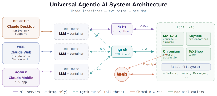
This started as a plumbing problem. I wanted to move files between Claude’s cloud container and my Mac faster than base64 encoding allows. What I ended up building was something more interesting: a way for every Claude – Desktop, web browser, iPhone – to control my entire computing environment with natural language. MATLAB, Keynote, LaTeX, Chrome, Safari, my file system, text-to-speech. All of it, from any device, through a 200-line Python server and a free tunnel.
It isn’t quite the ideal universal remote. Web and iPhone Claude do not yet have the agentic Playwright-based web automation capabilities available to Claude desktop via MCP. A possible solution may be explored in a later post.
Background information
The background here is a series of experiments I’ve been running on giving AI desktop apps direct access to local tools. See How to set up and use AI Desktop Apps with MATLAB and MCP servers which covers the initial MCP setup, A universal agentic AI for your laptop and beyond which describes what Desktop Claude can do once you give it the keys, and Web automation with Claude, MATLAB, Chromium, and Playwright which describes a supercharged browser assistant. This post is about giving such keys to remote Claude interfaces.
Through the Model Context Protocol (MCP), Claude Desktop on my Mac can run MATLAB code, read and write files, execute shell commands, control applications via AppleScript, automate browsers with Playwright, control iPhone apps, and take screenshots. These powers have been limited to the desktop Claude app – the one running on the machine with the MCP servers. My iPhone Claude app and a Claude chat launched in a browser interface each have a Linux container somewhere in Anthropic’s cloud. The container can reach the public internet. Until now, my Mac sat behind a home router with no public IP.
An HTTP server MCP replacement
A solution is a small HTTP server on the Mac. Use ngrok (free tier) to give the Mac a public URL. Then anything with internet access – including any Claude’s cloud container – can reach the Mac via curl.
iPhone/Web Claude -> bash_tool: curl https://public-url/endpoint
-> Internet -> ngrok tunnel -> Mac localhost:8765
-> Python command server -> MATLAB / AppleScript / filesystem
The server is about 200 lines of Python using only the standard library. Two files, one terminal command to start. ngrok provides HTTPS and HTTP Basic Auth with a single command-line flag.
The complete implementation consists of three files:
claude_command_server.py (~200 lines): A Python HTTP server using http.server from the standard library. It implements BaseHTTPRequestHandler with do_GET and do_POST methods dispatching to endpoint handlers. Shell commands are executed via subprocess.run with timeout protection. File paths are validated against allowed roots using os.path.realpath to prevent directory traversal attacks.
start_claude_server.sh (~20 lines): A Bash script that starts the Python server as a background process, then starts ngrok in the foreground. A trap handler ensures both processes are killed on Ctrl+C.
iphone_matlab_watcher.m (~60 lines): MATLAB timer function that polls for command files every second.
The server exposes six GET and six POST endpoints. The GET endpoints thus far handle retrieval: /ping for health checks, /list to enumerate files in a transfer directory, /files/<n> to download a file from that directory, /read/<path> to read any file under allowed directories, and / which returns the endpoint listing itself. The POST endpoints handle execution and writing: /shell runs an allowlisted shell command, /osascript runs AppleScript, /matlab evaluates MATLAB code through a file-watcher mechanism, /screenshot captures the screen and returns a compressed JPEG, /write writes content to a file, and /upload/<n> accepts binary uploads.
File access is sandboxed by endpoint. The /read/ endpoint restricts reads to ~/Documents, ~/Downloads, and ~/Desktop and their subfolders. The /write and /upload endpoints restrict writes to ~/Documents/MATLAB and ~/Downloads. Path traversal is validated – .. sequences are rejected.
The /shell endpoint restricts commands to an explicit allowlist: open, ls, cat, head, tail, cp, mv, mkdir, touch, find, grep, wc, file, date, which, ps, screencapture, sips, convert, zip, unzip, pbcopy, pbpaste, say, mdfind, and curl. No rm, no sudo, no arbitrary execution. Content creation goes through /write.
Two endpoints have no path restrictions: /osascript and /matlab. The /osascript endpoint passes its payload to macOS’s osascript command, which executes AppleScript – Apple’s scripting language for controlling applications via inter-process Apple Events. An AppleScript can open, close, or manipulate any application, read or write any file the user account can access, and execute arbitrary shell commands via “do shell script”. The /matlab endpoint evaluates arbitrary MATLAB code in a persistent session. Both are as powerful as the user account itself. This is deliberate – these are the endpoints that make the server useful for controlling applications. The security boundary is authentication at the tunnel, not restriction at the endpoint.
The MATLAB Workaround
MATLAB on macOS doesn’t expose an AppleScript interface, and the MCP MATLAB tool uses a stdio connection available only from Desktop. So how does iPhone Claude run MATLAB?
An answer is a file-based polling mechanism. A MATLAB timer function checks a designated folder every second for new command files. The remote Claude writes a .m file via the server, MATLAB executes it, writes output to a text file, and sets a completion flag. The round trip is about 2.5 seconds including up to 1 second of polling latency. (This could be reduced by shortening the polling interval or replacing it with Java’s WatchService for near-instant file detection.)
This method provides full MATLAB access from a phone or web Claude, with your local file system available, under AI control. MATLAB Mobile and MATLAB Online do not offer agentic AI access.
Alternate approaches
I’ve used Tailscale Funnel as an alternative tunnel to manually control my MacBook from iPhone but you can’t install Tailscale inside Anthropic’s container. An alternative approach would replace both the local MCP servers and the command server with a single remote MCP server running on the Mac, exposed via ngrok and registered as a custom connector in claude.ai. This would give all three Claude interfaces native MCP tool access including Playwright or Puppeteer with comparable latency but I’ve not tried this.
Security
Exposing a command server to the internet raises questions. The security model has several layers. ngrok handles authentication – every request needs a valid password. Shell commands are restricted to an allowlist (ls, cat, cp, screencapture – no rm, no arbitrary execution). File operations are sandboxed to specific directory trees with path traversal validation. The server binds to localhost, unreachable without the tunnel. And you only run it when you need it.
The AppleScript and MATLAB endpoints are relatively unrestricted in my setup, giving Claude Desktop significant capabilities via MCP. Extending them through an authenticated tunnel is a trust decision.
Initial test results
I ran an identical three-step benchmark from each Claude interface: get a Mac timestamp via AppleScript, compute eigenvalues of a 10x10 magic square in MATLAB, and capture a screenshot. Same Mac, same server, same operations.
| Step | Desktop (MCP) | Web Claude | iPhone Claude |
|------|:------------:|:----------:|:-------------:|
| AppleScript timestamp | ~5ms | 626ms | 623ms |
| MATLAB eig(magic(10)) | 108ms | 833ms | 1,451ms |
| Screenshot capture | ~200ms | 1,172ms | 980ms |
| **Total** | **~313ms** | **2,663ms** | **3,078ms** |
The network overhead is consistent: web and iPhone both add about 620ms per call (the ngrok round trip through residential internet). Desktop MCP has no network overhead at all. The MATLAB variance between web (833ms) and iPhone (1,451ms) is mostly the file-watcher polling jitter – up to a second of random latency depending on where in the polling cycle the command arrives.
All three Claudes got the correct eigenvalues. All three controlled the Mac. The slowest total was 3 seconds for three separate operations from a phone. Desktop is 10x faster, but for “I’m on my phone and need to run something” – 3 seconds is fine.
Other tests
MATLAB: Computations (determinants, eigenvalues), 3D figure generation, image compression. The complete pipeline – compute on Mac, transfer figure to cloud, process with Python, send back – runs in under 5 seconds. This was previously impossible; there was no reasonable mechanism to move a binary file from the container to the Mac.
Keynote: Built multi-slide presentations via AppleScript, screenshotted the results.
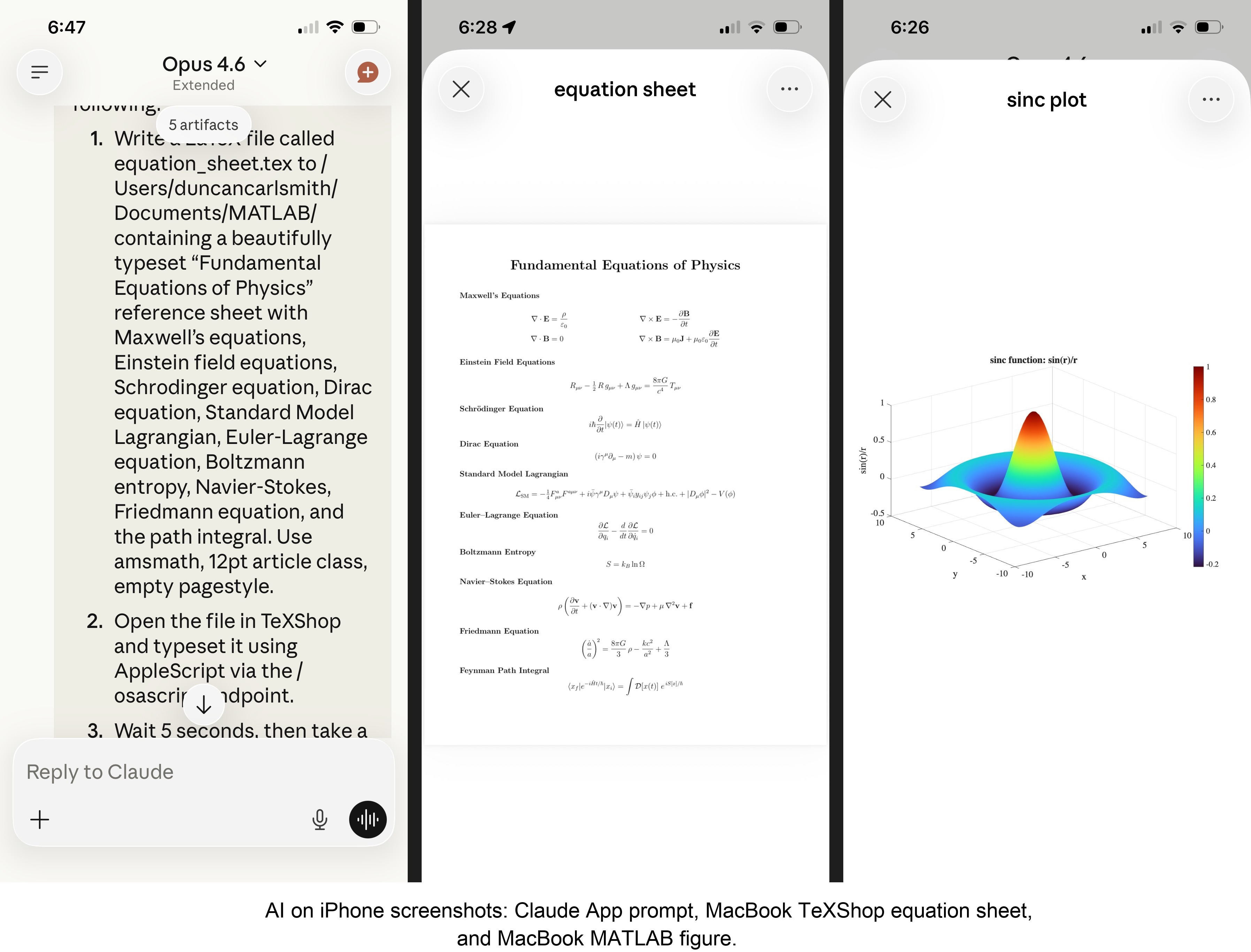
TeXShop: Wrote a .tex file containing ten fundamental physics equations (Maxwell through the path integral), opened it in TeXShop, typeset via AppleScript, captured the rendered PDF. Publication-quality typesetting from a phone. I don’t know who needs this at 11 PM on a Sunday, but apparently I do.
Safari: Launched URLs on the Mac from 2,000 miles away. Or 6 feet. The internet doesn’t care.
Finder: Directory listings, file operations, the usual filesystem work.
Text-to-speech: Mac spoke “Hello from iPhone” and “Web Claude is alive” on command. Silly but satisfying proof of concept.
File Transfer: The Original Problem, Solved
Remember, this started because I wanted faster file transfers for desktop Claude. Compare:
| Method | 1 MB file | 5 MB file | Limit |
|--------|-----------|-----------|-------|
| Old (base64 in context) | painful | impossible | ~5 KB |
| Command server upload | 455ms | ~3.6s | tested to 5 MB+ |
| Command server download | 1,404ms | ~7s | tested to 5 MB+ |
The improvement is the difference between “doesn’t work” and “works in seconds.”
Cross-Device Memory
A nice bonus: iPhone and web Claudes can search Desktop conversations using the same memory tools. Context established in a Desktop session – including the server password – can be retrieved from a phone conversation. You do have to ask explicitly (“search my past conversations for the command server”) or insert information into the persistent context using settings rather than assuming Claude will look on its own.
Web Claudes
The most surprising result was web Claude. I expected it to work – same container infrastructure, same bash_tool, same curl. But “expected to work” and “just worked, first try, no special setup” are different things. I opened claude.ai in a browser, gave it the server URL and password, and it immediately ran MATLAB, took screenshots, and made my Mac speak. No configuration, no troubleshooting, no “the endpoint format is wrong” iterations. If you’re logged into claude.ai and the server is running, you have full Mac access from any browser on any device.
What This Means
MCP gave Desktop Claude the keys to my Mac. A 200-line server and a free tunnel duplicated those keys for every other Claude I use. Three interfaces, one Mac, all the same applications, all controlled in natural language.
Additional information
An appendix gives Claude’s detailed description of communications. Codes and instructions are available at the MATLAB File Exchange: Giving All Your Claudes the Keys to Everything.
Acknowledgments and disclaimer
The problem of file transfer was identified by the author. Claude suggested and implemented the method, and the author suggested the generalization to accommodate remote Claudes. This submission was created with Claude assistance. The author has no financial interest in Anthropic or MathWorks.
—————
Appendix: Architecture Comparison
Path A: Desktop Claude with a Local MCP Server
When you type a message in the Desktop Claude app, the Electron app sends it to Anthropic’s API over HTTPS. The LLM processes the message and decides it needs a tool – say, browser_navigate from Playwright. It returns a tool_use block with the tool name and arguments. That block comes back to the Desktop app over the same HTTPS connection.
Here is where the local MCP path kicks in. At startup, the Desktop app read claude_desktop_config.json, found each MCP server entry, and spawned it as a child process on your Mac. It performed a JSON-RPC initialize handshake with each one, then called tools/list to get the tool catalog – names, descriptions, parameter schemas. All those tools were merged and sent to Anthropic with your message, so the LLM knows what’s available.
When the tool_use block arrives, the Desktop app looks up which child process owns that tool and writes a JSON-RPC message to that process’s stdin. The MCP server (Playwright, MATLAB, whatever) reads the request, does the work locally, and writes the result back to stdout as JSON-RPC. The Desktop app reads the result, sends it back to Anthropic’s API, the LLM generates the final text response, and you see it.
The Desktop app is really just a process manager and JSON-RPC router. The config file is a registry of servers to spawn. You can plug in as many as you want – each is an independent child process advertising its own tools. The Desktop app doesn’t care what they do internally. The MCP execution itself adds almost no latency because it’s entirely local, process-to-process on your Mac. The time you perceive is dominated by the two HTTPS round-trips to Anthropic, which all three Claude interfaces share equally.
Path B: iPhone Claude with the Command Server
When you type a message in the Claude iOS app, the app sends it to Anthropic’s API over HTTPS, same as Desktop. The LLM processes the message. It sees bash_tool in its available tools – provided by Anthropic’s container infrastructure, not by any MCP server. It decides it needs to run a curl command and returns a tool_use block for bash_tool.
Here, the path diverges completely from Desktop. There is no iPhone app involvement in tool execution. Anthropic routes the tool_use to a Linux container running in Anthropic’s cloud, assigned to your conversation. This container is the “computer” that iPhone Claude has access to. The container runs the curl command – a real Linux process in Anthropic’s data center.
The curl request goes out over the internet to ngrok’s servers. ngrok forwards it through its persistent tunnel to the claude_command_server.py process running on localhost on your Mac. The command server authenticates the request (basic auth), then executes the requested operation – in this case, running an AppleScript via subprocess.run(['osascript', ...]). macOS receives the Apple Events, launches the target application, and does the work.
The result flows back the same way: osascript returns output to the command server, which packages it as JSON and sends the HTTP response back through the ngrok tunnel, through ngrok’s servers, back to the container’s curl process. bash_tool captures the output. The container sends the tool result back to Anthropic’s API. The LLM generates the text response, and the iPhone app displays it.
The iPhone app is a thin chat client. It never touches tool execution – it only sends and receives chat messages. The container does the curl work, and the command server bridges from Anthropic’s cloud to your Mac. The LLM has to know to use curl with the right URL, credentials, and JSON format. There is no tool discovery, no protocol handshake, no automatic routing. The knowledge of how to reach your Mac is carried entirely in the LLM’s context.
—————
Duncan Carlsmith, Department of Physics, University of Wisconsin-Madison. duncan.carlsmith@wisc.edu
Hi everyone,
Simulations have a way of outgrowing the machine they run on (at least mine do). Bigger sweeps, longer regression suites, more data to pull in. At some point your workstation just isn't beefy enough!
I've just published a post on running larger MATLAB and Simulink simulations in the cloud (e.g. AWS): more compute when we need it, without changing how we work day to day.
The example is from automotive, but the same applies to aerospace, robotics, and beyond.
If you want to read more, here's the link: https://blogs.mathworks.com/engineering/2026/07/14/on-scaling-model-based-design-into-the-cloud/
How are others handling scaling for simulation? what's working for you?
Cheers,
George
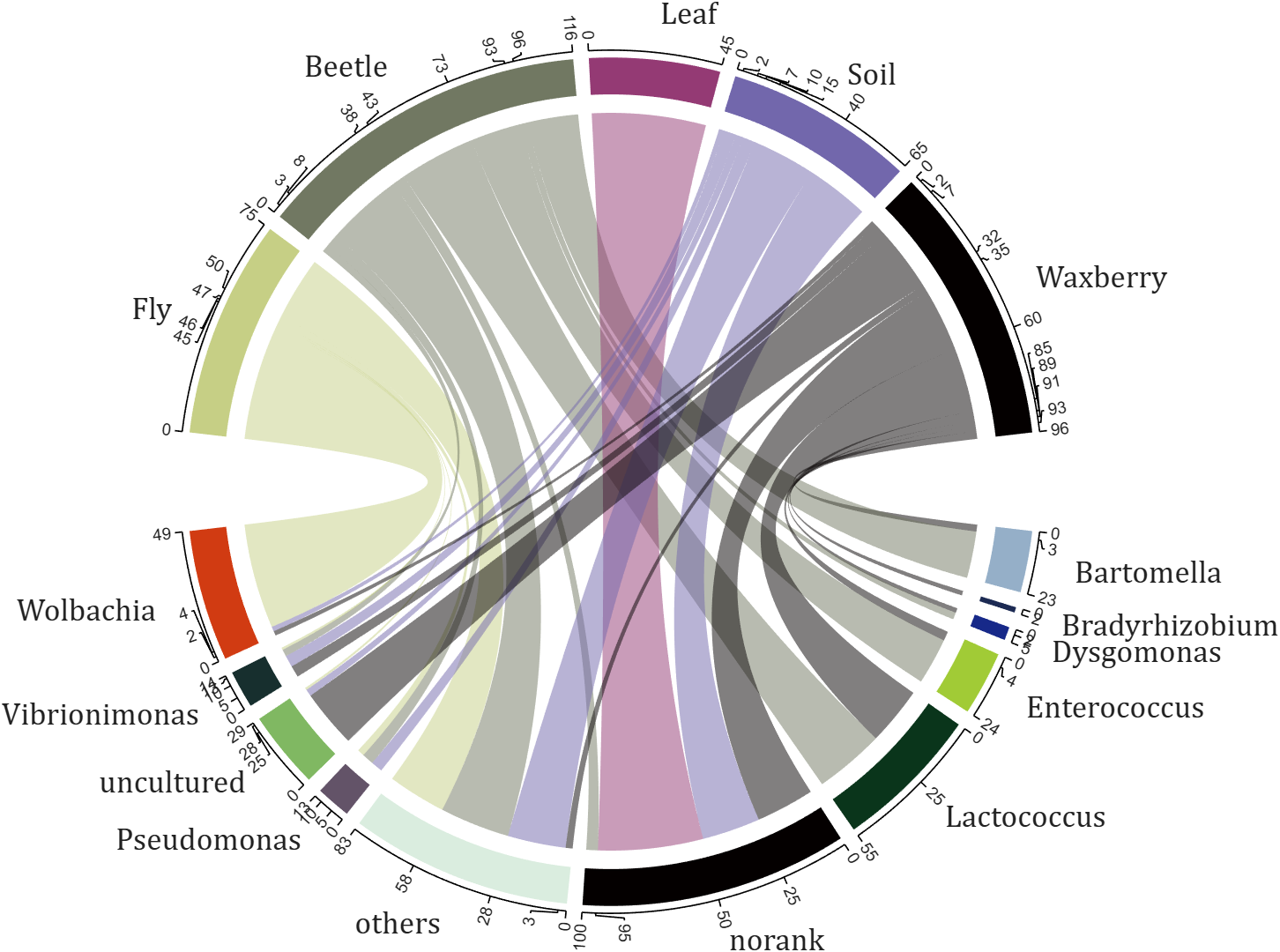
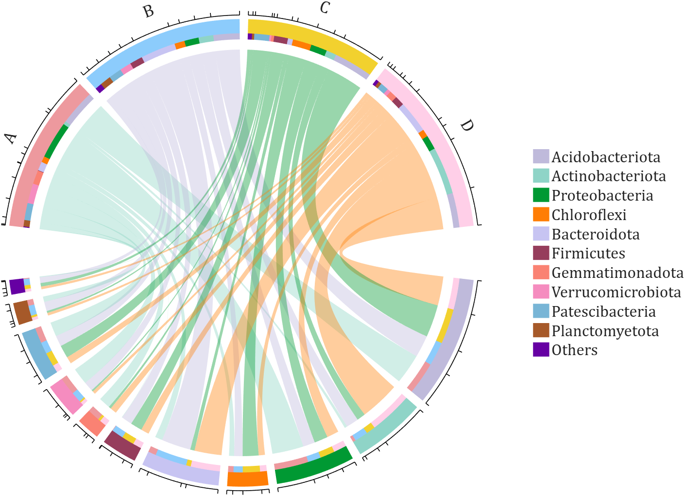
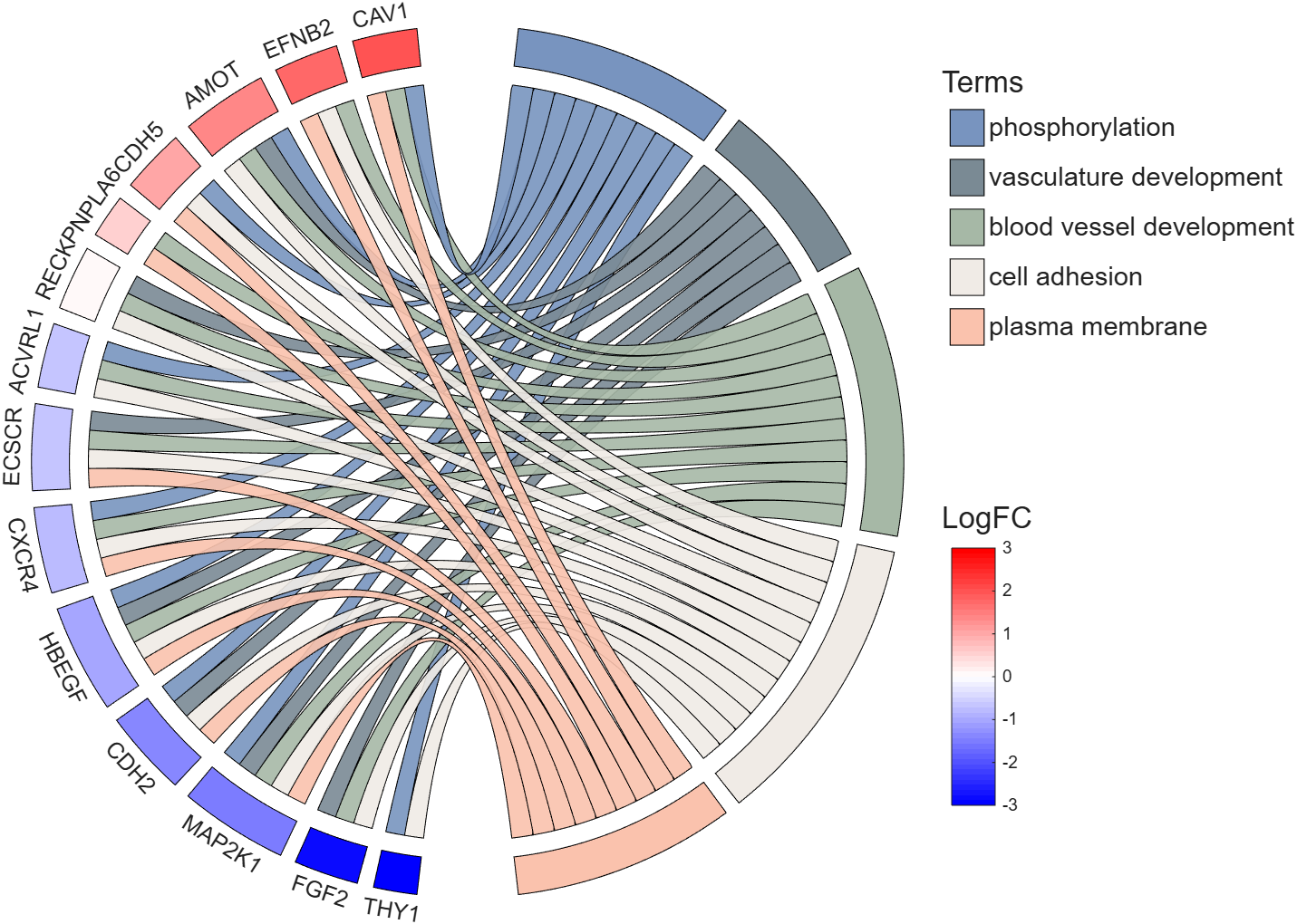
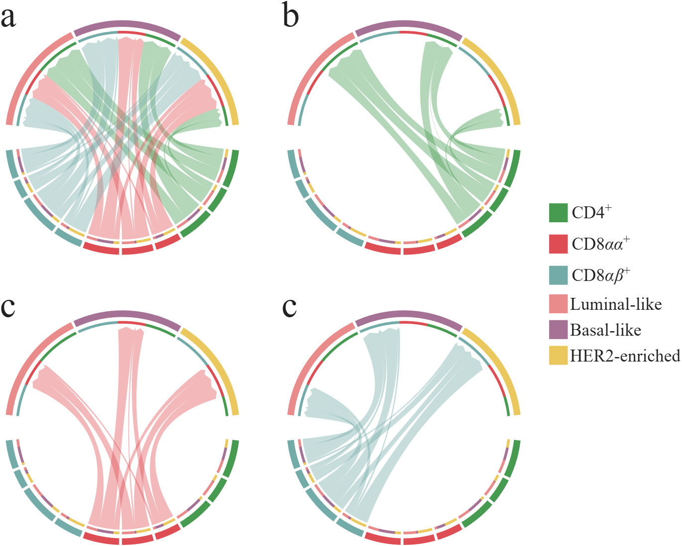
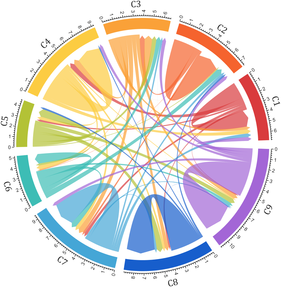
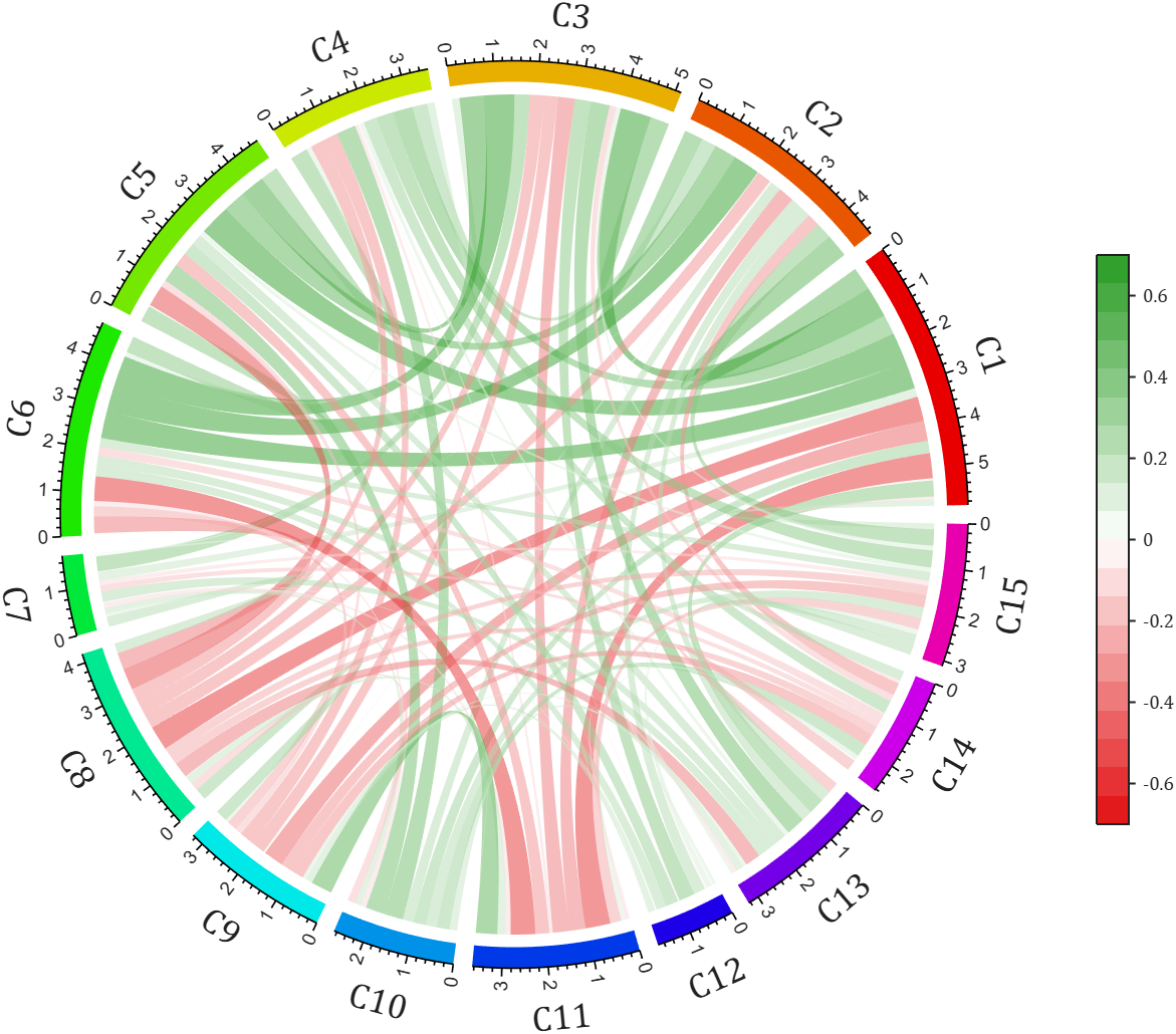
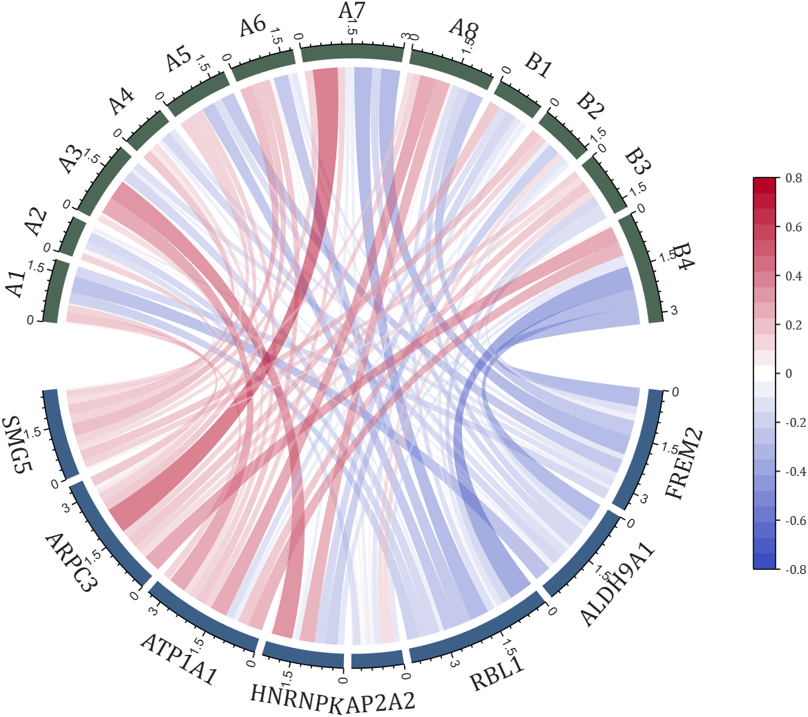
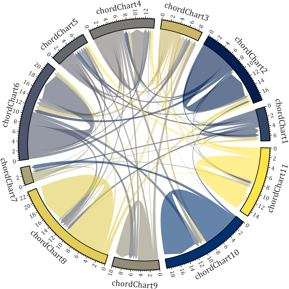
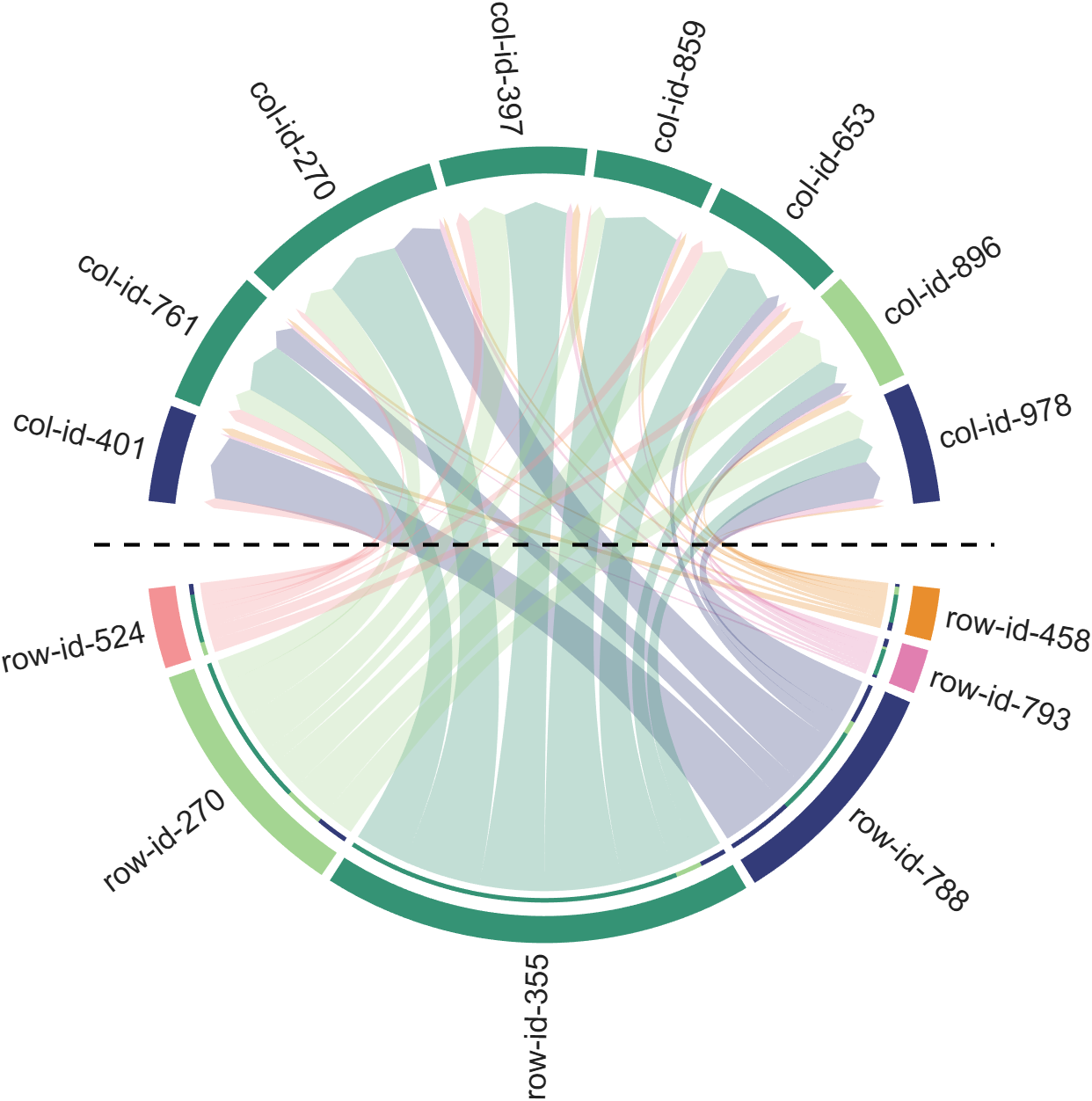
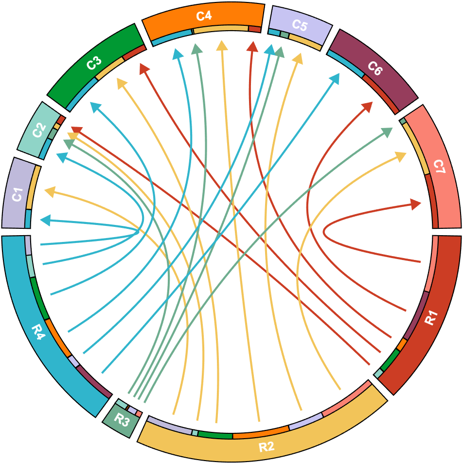
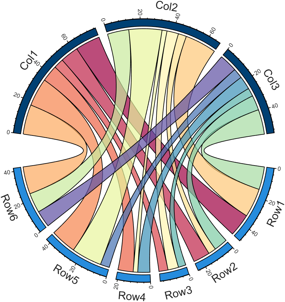
All figures presented in this Discussion were generated using MATLAB.
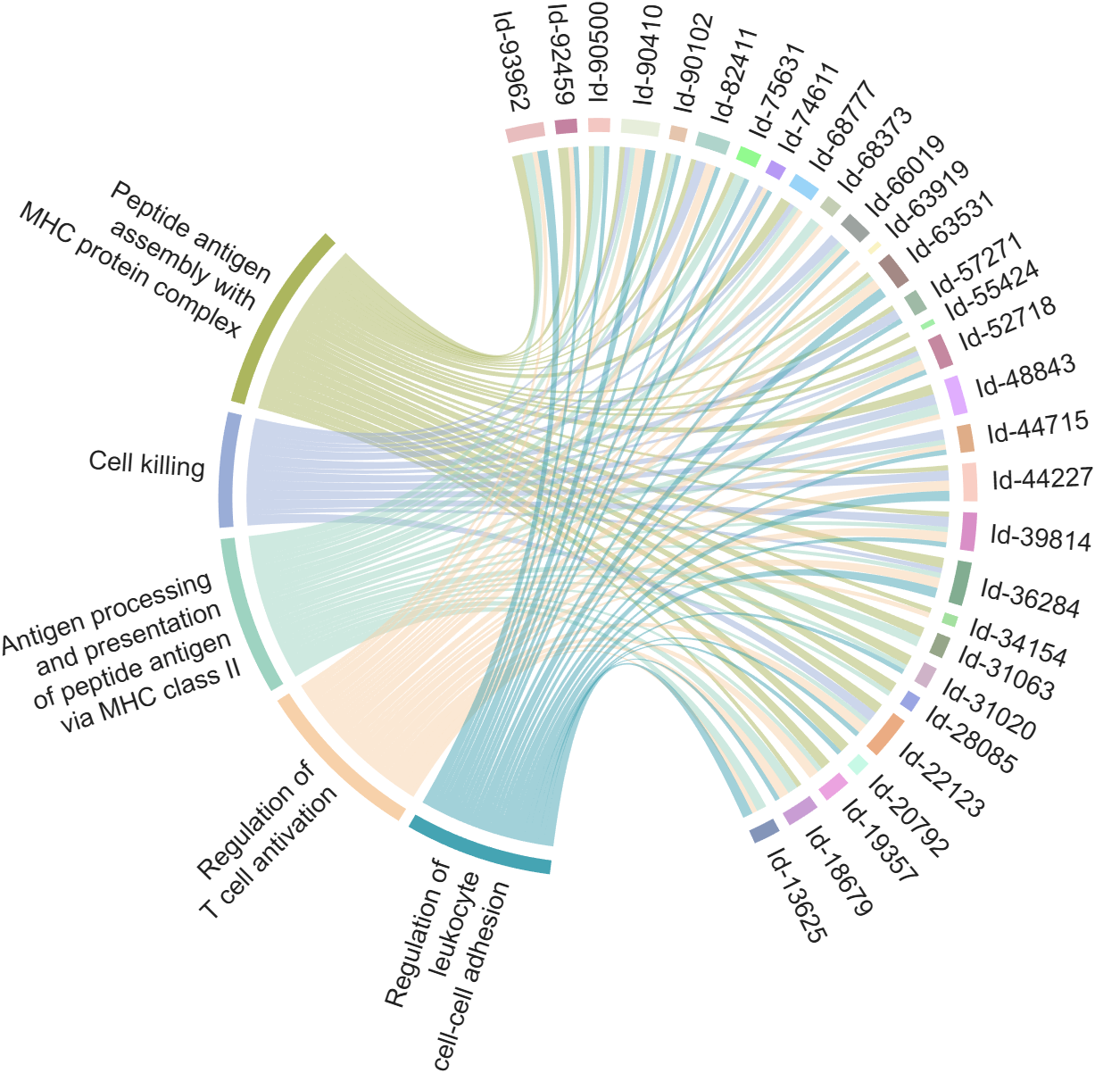
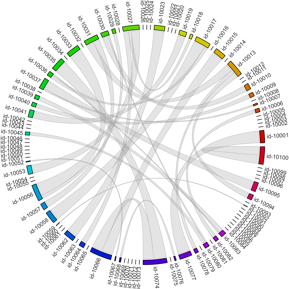
I developed two functions: one for plotting chord diagrams without self-loops, and the other for plotting chord diagrams with self-loops.
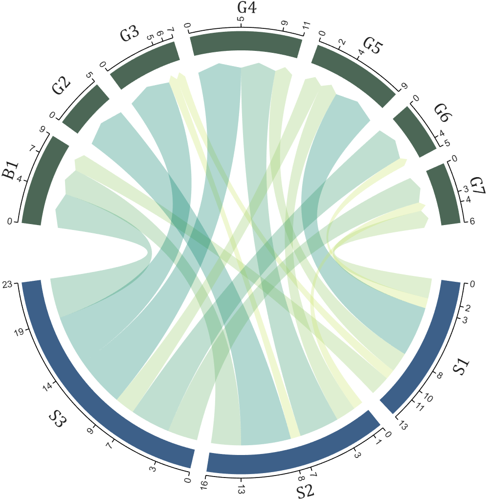
chordChart : basic usage
plotting chord diagrams without self-loops : https://www.mathworks.com/matlabcentral/fileexchange/116550-chordchart-chord-diagram
dataMat = [2 0 1 2 5 1 2;
3 5 1 4 2 0 1;
4 0 5 5 2 4 3];
colName = {'B1','G2','G3','G4','G5','G6','G7'};
rowName = {'S1','S2','S3'};
% Create and render chord diagram object (创建弦图对象并渲染)
CC = chordChart(dataMat, 'RowName',rowName, 'ColName',colName, 'Arrow','on');
CC.LinearMinorTick = 'on';
CC.draw();
% Set Font for labels and show ticks (调整字体并显示刻度)
CC.setFont('FontSize',17, 'FontName','Cambria')
CC.tickState('on')
CC.tickLabelState('on')
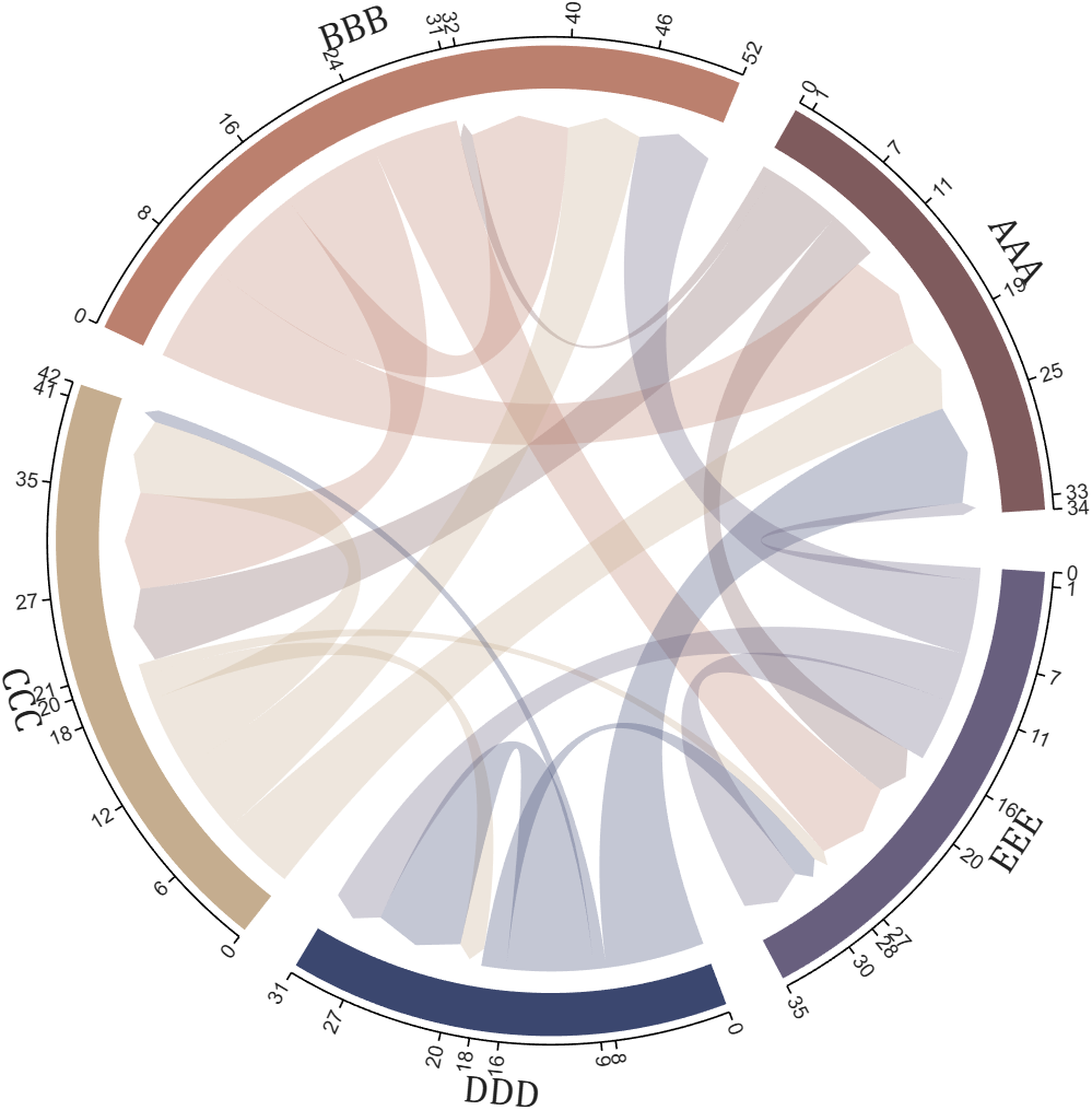
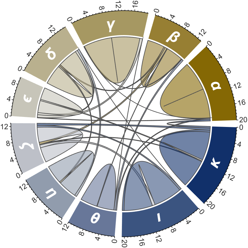
biChordChart : basic usage
plotting chord diagrams with self-loops : https://www.mathworks.com/matlabcentral/fileexchange/121043-bichordchart-bidirectional-chord-diagram
dataMat = randi([0,8], [5,5]);
nameList = {'AAA','BBB','CCC','DDD','EEE'};
% Create bichord chart object and draw (创建并绘制双向弦图对象)
BCC = biChordChart(dataMat, 'Arrow','on', 'Label',nameList);
BCC = BCC.draw();
% Show ticks and tick labels (添加刻度)
BCC.tickState('on')
BCC.tickLabelState('on')
% Set font properties (修改字体,字号及颜色)
BCC.setFont('FontName','Cambria','FontSize',17)
The two File Exchange submissions each provide more than a dozen basic examples. In addition, the GitHub repository listed below provides nearly 40 elaborate customized demonstration cases.
MATLAB Editor (built-in editor)
74%
VS Code (Visual Studio Code)
18%
Jupyter Notebook / MATLAB Kernel
2%
PyCharm (via plugins or external )
2%
Sublime Text / Atom
1%
Others (please specify in commets)
2%
960 votes
Looking for an on-campus job next semester? We’re hiring MATLAB Student Ambassadors to host fun events, share MATLAB resources on social media, and connect with your student community.
Learn more here: https://www.mathworks.com/academia/students/student-ambassadors.html

How does everyone use MatLab right now? I can't think of any ideas what i can use this software for!
Hi everyone
It is my pleasure to be able to report on a project that several teams at MathWorks have been working on for some time now. A new object management system that promises to make object oriented code in MATLAB a lot faster.
The new system is available as a limited beta in the pre-release of MATLAB 2026b. It is not turned on by default. If you are developing OOP code, we'd love you to try it out. Most of the time, no code changes will be necessary but there are a small number of well-defined case where you will need to update your code.
The team are currently looking for MATLAB developers to work with who would like to try this out.
More details, including how to join the beta, are available in the following blog post https://blogs.mathworks.com/matlab/2026/07/14/objects-are-about-to-get-much-faster-in-matlab/
Best wishes,
Mike
Did you know that function double with string vector input significantly outperforms str2double with the same input:
x = rand(1,50000);
t = string(x);
tic; str2double(t); toc
tic; I1 = str2double(t); toc
tic; I2 = double(t); toc
isequal(I1,I2)
Recently I needed to parse numbers from text. I automatically tried to use str2double. However, profiling revealed that str2double was the main bottleneck in my code. Than I realized that there is a new note (since R2024a) in the documentation of str2double:
"Calling string and then double is recommended over str2double because it provides greater flexibility and allows vectorization. For additional information, see Alternative Functionality."
I have been a loyal MATLAB user for 25 years, starting from my university days. While many of my peers migrated to Python, I stayed for the stability, compatibility, and clean environment. However, I am finding the 2025 version exceptionally laggy. Despite running it on an $10k high-end machine, simple tasks like viewing variables and plotting take up to 60 seconds - actions that were near instantaneous in the 2020 version. I want to stay continue with MATLAB, but this performance gap is a major hurdle and irritation. I hope these optimization issues can be addressed quickly.
Many widely cited code style guides originate from large-scale software engineering contexts: multi-developer teams, large codebases, separate reviewers, and tooling-driven workflows. While those constraints are valid in their domain, they often map poorly onto scientific and engineering scripting as it is typically practiced with MATLAB.
In laboratory and engineering environments, code serves a different role. It is frequently written by individuals or small groups, and then iteratively modified, copied, adapted, and extended as part of an evolving problem-solving process. In this context, the primary priorities are not strict stylistic consistency or tooling compatibility, but rather:
- maintaining clarity of underlying structure,
- minimizing the risk of errors during modification, and
- supporting rapid comprehension of mathematically or logically dense code.
This raises the question: should fixed line-length limits be replaced by context-aware principles? Could these be supported by a suitable AI tool?
The following proposal outlines a small set of heuristics governing line length, based on observations of real-world MATLAB usage, particularly for numerically intensive and structurally rich code. These heuristics aim to:
- preserve and expose meaningful structure (e.g. systems of equations, tables, repeated patterns)
- avoid formatting that obscures relationships or introduces errors, and
- treat different kinds of code (logic vs. data vs. structured expressions) appropriately.
Scope
These principles apply to scientific and engineering scripting, particularly:
- MATLAB-like environments
- numerically or structurally dense code
- monolithic or semi-monolithic workflows
- code that is frequently modified, copied, and adapted
They are not intended for large-scale commercial software engineering, where different constraints dominate.
Core Objective
Line length and formatting should maximize comprehension, structural clarity, and correctness under modification, rather than enforce arbitrary limits.
Hierarchy of Heuristics
Higher-numbered heuristics take precedence over lower-numbered ones.
1) Reasonable Line Length
Code intended for reading should use a reasonable line length, guided by:
- human visual comprehension when scanning
- clarity of expression
- preservation of logical units
This would tend toward 70-100 characters per line, depending on the density.
2) Preserve Semantic Integrity of Lines
Line breaks must not split code in ways that degrade understanding.
Avoid:
- dangling fragments
- very short continuation lines
- separation of tightly coupled elements
- etc.
Prefer:
- keeping logically cohesive expressions intact
- breaking only at clear structural boundaries
One slightly longer line is preferable to two poorly structured lines.
3) Treat Data as Data (Not Prose/Code)
Code that primarily represents data rather than logic is not intended for sequential reading.
This includes:
- large numeric vectors
- lookup tables
- pasted datasets
- etc.
Such code:
- may exceed line length limits without restriction
- should prioritize density and structural stability
- is assumed to be accessed via search or indexing rather than visual parsing
Readability is not the objective; retrievability and integrity are. Yes, this intentionally rejects the enterprise concept that data must be separate from code, instead replacing it with the concept that the IDE should support what some real-world users actually use, for example by formatting/aligning/showing data differently.
4) Preserve and Expose 2D Structure
If code encodes a logical, mathematical, or tabular structure with inherent spatial relationships, it should be represented accordingly.
This includes:
- systems of equations
- tabulated data
- repeated structured expressions
- etc.
Requirements:
- alignment should be used where it improves comprehension
- patterns should be visually apparent
- deviations from patterns should be easily detectable
This principle should be applied strongly, tending toward mandatory use where feasible.
Exception
If a structure would become impractically wide, a compromise representation may be used.
Breaking meaningful spatial structure is considered harmful to comprehension and correctness.
5) Preserve Structural Consistency Across Similar Code
Code segments representing similar or related logic should be expressed in consistent structure and layout.
This applies to:
- repeated formulas
- analogous computations
- structurally similar transformations
- etc.
Consistency enables:
- rapid comparison
- detection of inconsistencies
- safer modification
Similar logic should be represented in similar ways.
Meta-Principles
A. Structure Over Style
Line lengths should reflect the underlying structure of the problem, not conform to arbitrary limits.
B. Correctness Over Convention
Avoid line lengths and formatting that:
- obscures patterns
- hides inconsistencies
- increases the risk of modification errors
C. Optimize for Modification
Code in this domain is frequently:
- edited
- duplicated
- adapted for n
- extended
- commented-out for testing different versions
- etc
Line lengths should reduce the likelihood of errors during these operations, for example by keeping atomic concepts on the same line rather than splitting them up.
D. Anomaly Visibility
Formatting should make unexpected deviations immediately visible.
E. Tool Support
An intelligent tool should:
- respect and preserve structural layout
- avoid rigid line-length enforcement
- detect patterns and inconsistencies
- assist rather than constrain the programmer
I would be interested to hear how well these ideas match others’ experience, particularly in scientific or engineering workflows.
See also:
Hallo zusammen,
Ich habe einen Frage zu meinen Programm. Dies will einfach nicht laufen und ich finde keinen Fehler mehr. Ich habe mein Programm bei Simulink geschriebenen den Code bei Maltab Function. Das Board ist ein Adruino Uni Board. Ein Ultrasonic Sensor soll die Füllstände ich Wäschekörben messen. Dabei wird unter voll oder halbvoll entschieden. Anschließend wird ein Motor angesprochen, der entweder 15 oder 30 Sekunden laufen soll. Überwacht wird der Motor von einem Thermistor (den habe ich hier PT100 genannt) und einen Vibrationsschalter. Dazu soll der Vibrationsschalter über einen Resetknopf zurückgesetzt werden. Ich hoffe ihr könnt mir weiterhelfen.
Vielen Dank:)
if true
% code
end
n= input('Escolhe um número inteiro postivo. ')
primo=true;
i=2;
while i<n
if mod(n,i)==0;
primo=false;
end
i= i+1;
end
if primo && n>1;
disp('É primo')
else
disp('Não é primo')
end
anterior= n-1;
while true
primo=true;
i=2;
while i< anterior
if mod(anterior,i)==0;
primo= false;
end
i= i+1;
end
if primo && anterior>1;
end
anterior= anterior-1;
end
disp(anterior)
seguinte= n+1;
while true;
primo= true;
i=2;
while i<seguinte;
if mod(seguinte,i)==0;
primo=false;
end
i=i+1;
end
if primo && seguinte>1;
end
seguinte= seguinte+1;
end
disp(seguinte)
Any ideas? It is in portuguese if you intend to translate it.
How does MATLAB ThingSpeak Work ?
I spent some time tonight updating the UIHTML App skills on the MATLAB Agent Skills Playground hosted on GitHub.
We are using this repo to share early ideas and experiments with agent skills.
I submitted a Matlab support case but posting this publicly to hopefully save people some trouble and see if anyone has ideas.
After upgrading my workstation from Ubuntu 25.10 to Ubuntu 26.04 LTS, MATLAB GUI consistently prints this terminal error on shutdown:
free(): chunks in smallbin corrupted
MATLAB appears to run normally, but closing the GUI takes a long time and sometimes produces crash dumps. The terminal error occurs every time I close the GUI, but crash dumps are intermittent. I attached one R2026a crash dump. I had zero issues on Ubuntu 25.10.
Affected versions:
- MATLAB R2026a
- MATLAB R2025b
- I suspect any 'new desktop' version
System:
- Ubuntu 26.04 LTS
- AMD EPYC 7443P
- NVIDIA RTX 3090
- Ubuntu 26.04 default NVIDIA driver: nvidia-driver-595-open, 595.58.03
- NVIDIA module path: /lib/modules/7.0.0-14-generic/kernel/nvidia-595-open/nvidia.ko
- glibc 2.43
Important note: the error first occurred with a clean MathWorks MATLAB installation before installing the Ubuntu/Debian `matlab-support` package. I later tested after installing `matlab-support`, which I understand modifies/renames some MATLAB-bundled libraries so MATLAB uses selected system libraries instead. The same shutdown error occurs both before and after applying `matlab-support`. This suggests the issue is not caused solely by the Debian/Ubuntu `matlab-support` integration or solely by one of the libraries it substitutes.
The attached crash dump shows abort/free() heap corruption detected in libc, but the higher-level stack includes MATLAB libraries such as:
- libmwcppmicroservices.so
- libmwmodule_descriptor_implementation.so
- libmwmatlab_main_lib.so
- libmwfoundation_threadpool.so
The issue appears GUI-specific. Using these startup flags shut down cleanly:
- matlab -batch
- matlab -nodesktop
- matlab -nodisplay
The shutdown error still occurs with these startup flags:
- normal GUI launch
- -nosplash
- -nojvm
- -softwareopengl
- -cefdisablegpu
The issue also persists after:
- renaming/resetting ~/.matlab/R2026a and ~/.MathWorks/R2026a
- launching with a clean environment without LD_LIBRARY_PATH, LD_PRELOAD, MATLAB_JAVA, JAVA_HOME, JRE_HOME, etc.
- testing a new Ubuntu user account
- testing Ubuntu/GNOME, GNOME, and Xfce X11 sessions
- testing NO_AT_BRIDGE=1 and GTK_USE_PORTAL=0
- temporarily moving ~/.MathWorks/ServiceHost
- testing GLIBC_TUNABLES=glibc.malloc.tcache_count=0
- trying to capture a system coredump with ulimit -c unlimited / coredumpctl; no system coredump was produced
Because R2025b and R2026a are both affected, terminal-only modes exit cleanly, the problem occurs across GNOME/Wayland and Xfce/X11, and the error occurred on a clean MATLAB install before any `matlab-support` modifications, this appears related to MATLAB GUI shutdown on Ubuntu 26.04 / glibc 2.43 rather than a corrupted MATLAB preference folder, a single desktop session, or the Ubuntu `matlab-support` package.
Example crash dump:
When you are trying to bring the latest update into a coding like Codex, you can point the agent at a secret file called "llms.txt" -- this is file optimized for coding agents. I use it to over come "training data" bias. As even the latest models have outdated doc. This is important for working with projects that up date frequently.
Here are some of my favorites to use:
MATLAB AI Agent SDK lets you build and run AI agents in MATLAB.
- Create agents based on OpenAI®, Ollama™, or OpenAI-compatible APIs.
- Integrate LLMs and agentic workflows into your workflows in a targeted manner, retaining deterministic workflows when those are more suitable.
- Let your agent work on large amounts of data without needing to send the data to the LLM.
This SDK is a Research Preview under active development and APIs may change.
It turns out you can very easily change the list of verbs Claude Code uses to display when it's thinking. I've had fun replacing them with some MathWorks-specific verbiage. Comment below if you have any ideas to add to the list!
You just add the following to your settings.json file:
"spinnerVerbs": {
"mode": "replace",
"verbs": [
"MATLABing",
"Simulinking",
"MathWorking",
"MathWorkin' on it",
"Pre-allocating arrays",
"Checking 1-based indexing",
"Vectorizing",
"Eigenvaluing",
"FFT-ing",
"Transposing",
]
}
About Discussions
Discussions is a user-focused forum for the conversations that happen outside of any particular product or project.
Get to know your peers while sharing all the tricks you've learned, ideas you've had, or even your latest vacation photos. Discussions is where MATLAB users connect!
Get to know your peers while sharing all the tricks you've learned, ideas you've had, or even your latest vacation photos. Discussions is where MATLAB users connect!
More Community Areas

MATLAB Answers
Ask & Answer questions about MATLAB & Simulink!

File Exchange
Download or contribute user-submitted code!

Cody
Solve problem groups, learn MATLAB & earn badges!

Blogs
Get the inside view on MATLAB and Simulink!
AI Chat Playground
Use AI to generate initial draft MATLAB code, and answer questions!