predict
Predict responses for new observations from incremental drift-aware learning model
Since R2022b
Syntax
Description
[
also returns the classification scores, posterior probabilities, or the negated average
binary losses in yfit,m] = predict(___)m when Mdl.BaseLearner is an
incremental learning model for classification, using any of the input argument combinations
in the previous syntaxes. What m contains depends on the type of the
Mdl.BaseLearner model object.
Examples
Create the random concept data and the concept drift generator using the helper functions HelperRegrGenerator and HelperConceptDriftGenerator, respectively.
concept1 = HelperRegrGenerator(NumFeatures=100,NonZeroFeatures=[1,20,40,50,55], ...
    FeatureCoefficients=[4,5,10,-2,-6],NoiseStd=1.1,TableOutput=false);
concept2 = HelperRegrGenerator(NumFeatures=100,NonZeroFeatures=[10,20,45,56,80], ...
    FeatureCoefficients=[4,5,10,-2,-6],NoiseStd=1.1,TableOutput=false);
driftGenerator = HelperConceptDriftGenerator(concept1,concept2,15000,1000);
HelperRegrGenerator generates streaming data using features and feature coefficients for regression specified in the call to the function. At each step, the function samples the predictors from a normal distribution. Then, the function computes the response using the feature coefficients and predictor values and adding a random noise from a normal distribution with mean zero and specified noise standard deviation. The software returns the data in matrices for using in incremental learners.
HelperConceptDriftGenerator establishes the concept drift. The object uses a sigmoid function 1./(1+exp(-4*(numobservations-position)./width)) to decide the probability of choosing the first stream when generating data [3]. In this case, the position argument is 15000 and the width argument is 1000. As the number of observations exceeds the position value minus half of the width, the probability of sampling from the first stream when generating data decreases. The sigmoid function allows a smooth transition from one stream to the other. Larger width values indicate a larger transition period where both streams are approximately equally likely to be selected.
Initiate an incremental drift-aware model for regression as follows:
Create an incremental linear model for regression. Specify the linear regression model type and solver type.
Initiate an incremental concept drift detector that uses the Hoeffding's Bounds Drift Detection Method with moving average (HDDMA).
Using the incremental linear model and the concept drift detector, instantiate an incremental drift-aware model. Specify the training period as 6000 observations.
baseMdl = incrementalRegressionLinear(Learner="leastsquares",Solver="sgd",EstimationPeriod=1000,Standardize=false);
dd = incrementalConceptDriftDetector("hddma",Alternative="greater",InputType="continuous",WarmupPeriod=1000);
idaMdl = incrementalDriftAwareLearner(baseMdl,DriftDetector=dd,TrainingPeriod=6000);
Preallocate the number of variables in each chunk and the number of iterations for creating a stream of data.
numObsPerChunk = 10;
numIterations = 4000;
Preallocate the variables for tracking the drift status and drift time, and storing the regression error.
dstatus = zeros(numIterations,1);
statusname = strings(numIterations,1);
driftTimes = [];
ce = array2table(zeros(numIterations,2),VariableNames=["Cumulative" "Window"]);
Simulate a data stream with incoming chunks of 10 observations each and perform incremental drift-aware learning. At each iteration:
Simulate predictor data and labels, and update the drift generator using the helper function
hgenerate.Call
updateMetricsto update the performance metrics andfitto fit the incremental drift-aware model to the incoming data.Track and record the drift status and the regression error for visualization purposes.
rng(12); % For reproducibility

for j = 1:numIterations

 % Generate data
 [driftGenerator,X,Y] = hgenerate(driftGenerator,numObsPerChunk);

 % Update performance metrics and fit
 idaMdl = updateMetrics(idaMdl,X,Y);
 idaMdl = fit(idaMdl,X,Y);

 % Record drift status and regression error
 statusname(j) = string(idaMdl.DriftStatus);
 ce{j,:} = idaMdl.Metrics{"MeanSquaredError",:};
    if idaMdl.DriftDetected
       dstatus(j) = 2;
       driftTimes(end+1) = j;
    elseif idaMdl.WarningDetected
       dstatus(j) = 1;
    else
       dstatus(j) = 0;
    end

end
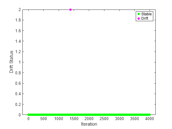
Plot the drift status versus the iteration number.
figure()
gscatter(1:numIterations,dstatus,statusname,'gmr','o',5,'on',"Iteration","Drift Status","filled")
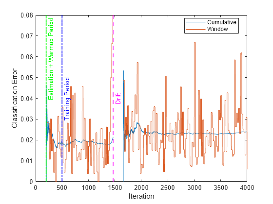
Plot the cumulative and per window regression error. Mark the warmup and training periods, and where the drift was introduced.
figure()
h = plot(ce.Variables);

xlim([0 numIterations])
ylim([0 20])
ylabel("Mean Squared Error")
xlabel("Iteration")

xline((idaMdl.MetricsWarmupPeriod+idaMdl.BaseLearner.EstimationPeriod)/numObsPerChunk,"g-.","Estimation Period + Warmup Period",LineWidth=1.5)
xline((idaMdl.MetricsWarmupPeriod+idaMdl.BaseLearner.EstimationPeriod)/numObsPerChunk+driftTimes,"g-.","Estimation Period + Warmup Period",LineWidth=1.5)
xline(idaMdl.TrainingPeriod/numObsPerChunk,"b-.","Training Period",LabelVerticalAlignment="middle",LineWidth=1.5)
xline(driftTimes,"m--","Drift",LabelVerticalAlignment="middle",LineWidth=1.5)

legend(h,ce.Properties.VariableNames)
legend(h,Location="best")

After the detection of drift, the fit function calls the reset function to reset the incremental drift-aware learner, hence the base learner and the drift detector. The updateMetrics function waits for idaMdl.BaseLearner.EstimationPeriod+idaMdl.MetricsWarmupPeriod observations to start updating model performance metrics again.
Generate new data. Reorient the predictor variables in columns.
[driftGenerator,X,Y] = hgenerate(driftGenerator,500);
X = X';
Predict responses on new data. Specify the orientation of the predictor variables.
yhat = predict(idaMdl,X,ObservationsIn="columns");Compute and plot the residuals.
res = Y - yhat;
plot(res)
ylabel("Residuals")
xlabel("New data points")

The residuals appear symmetrically spread around 0 for new data.
Create the random concept data using the HelperSineGenerator and concept drift generator HelperConceptDriftGenerator.
concept1 = HelperSineGenerator("ClassificationFunction",1,"IrrelevantFeatures",true,"TableOutput",false);
concept2 = HelperSineGenerator("ClassificationFunction",3,"IrrelevantFeatures",true,"TableOutput",false);
driftGenerator = HelperConceptDriftGenerator(concept1,concept2,15000,1000);
When ClassificationFunction is 1, HelperSineGenerator labels all points that satisfy x1 < sin(x2) as 1, otherwise the function labels them as 0. When ClassificationFunction is 3, this is reversed. That is, HelperSineGenerator labels all points that satisfy x1 >= sin(x2) as 1, otherwise the function labels them as 0.
HelperConceptDriftGenerator establishes the concept drift. The object uses a sigmoid function 1./(1+exp(-4*(numobservations-position)./width)) to decide the probability of choosing the first stream when generating data [1]. In this case, the position argument is 15000 and the width argument is 1000. As the number of observations exceeds the position value minus half of the width, the probability of sampling from the first stream when generating data decreases. The sigmoid function allows a smooth transition from one stream to the other. Larger width values indicate a larger transition period where both streams are approximately equally likely to be selected.
Instantiate an incremental drift-aware model as follows:
Create an incremental Naive Bayes classification model for binary classification.
Initiate an incremental concept drift detector that uses the Hoeffding's Bounds Drift Detection Method with moving average (HDDMA).
Using the incremental linear model and the concept drift detector, instantiate an incremental drift-aware model. Specify the training period as 5000 observations.
BaseLearner = incrementalClassificationLinear(Solver="sgd");
dd = incrementalConceptDriftDetector("hddma");
idaMdl = incrementalDriftAwareLearner(BaseLearner,DriftDetector=dd,TrainingPeriod=5000);
Preallocate the number of variables in each chunk and number of iterations for creating a stream of data.
numObsPerChunk = 10;
numIterations = 4000;
Preallocate the variables for tracking the drift status and drift time, and storing the classification error.
dstatus = zeros(numIterations,1);
statusname = strings(numIterations,1);
ce = array2table(zeros(numIterations,2),VariableNames=["Cumulative" "Window"]);
driftTimes = [];
Simulate a data stream with incoming chunks of 10 observations each and perform incremental drift-aware learning. At each iteration:
Simulate predictor data and labels, and update the drift generator using the helper function
hgenerate.Call
updateMetricsAndFitto update the performance metrics and fit the incremental drift-aware model to the incoming data.Track and record the drift status and the classification error for visualization purposes.
rng(12); % For reproducibility

for j = 1:numIterations

 % Generate data
 [driftGenerator,X,Y] = hgenerate(driftGenerator,numObsPerChunk);

 % Update performance metrics and fit
 idaMdl = updateMetricsAndFit(idaMdl,X,Y);

 % Record drift status and classification error
 statusname(j) = string(idaMdl.DriftStatus);
 ce{j,:} = idaMdl.Metrics{"ClassificationError",:};
 if idaMdl.DriftDetected
       dstatus(j) = 2;
       driftTimes(end+1) = j;
    elseif idaMdl.WarningDetected
       dstatus(j) = 1;
    else
       dstatus(j) = 0;
    end

end
Plot the cumulative and per window classification error. Mark the warmup and training periods, and where the drift was introduced.
h = plot(ce.Variables);

xlim([0 numIterations])
ylim([0 0.08])
ylabel("Classification Error")
xlabel("Iteration")

xline((idaMdl.BaseLearner.EstimationPeriod+idaMdl.MetricsWarmupPeriod)/numObsPerChunk,"g-.","Estimation + Warmup Period",LineWidth=1.5)
xline(idaMdl.TrainingPeriod/numObsPerChunk,"b-.","Training Period",LabelVerticalAlignment="middle",LineWidth=1.5)
xline(driftTimes,"m--","Drift",LabelVerticalAlignment="middle",LineWidth=1.5)

legend(h,ce.Properties.VariableNames)
legend(h,Location="best")
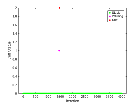
Plot the drift status versus the iteration number.
gscatter(1:numIterations,dstatus,statusname,'gmr','o',4,'on',"Iteration","Drift Status","Filled")
Generate new data of 500 observations. Predict class labels and classification scores for new data.
numnewdata = 500;
[driftGenerator,X,Y] = hgenerate(driftGenerator,numnewdata);
[yhat,cscores] = predict(idaMdl,X);
Compute ROC and plot the results.
roc = rocmetrics(Y,cscores,idaMdl.BaseLearner.ClassNames);
plot(roc)

For each class, the plot function plots a ROC curve and displays a filled circle marker at the model operating point. The legend displays the class name and AUC value for each curve. In a binary classification problem, the two ROC curves are symmetric, and the AUC values are identical.
Compute the accuracy of the model.
accuracy = sum(Y==yhat)/500
accuracy =
0.9780
The model predicts the new class labels with high accuracy.
Input Arguments
Output Arguments
References
Version History
Introduced in R2022b
See Also
fit | incrementalDriftAwareLearner | loss | updateMetrics | updateMetricsAndFit