Sliding Mode Control Design for Mass-Spring-Damper System
This example show how to implement sliding mode control (SMC) at the command line and in Simulink®. In this example, you implement SMC for a mass-spring-damper system.
Sliding Mode Control
In SMC, you define a sliding surface that the system state trajectory converges to and remains on. This sliding surface is designed such that it is insensitive to disturbances and uncertainties in the system. Once the system state trajectory is on the sliding surface, the controller uses a feedback control law to drive the system state trajectory to the desired state along the sliding surface. For more information, see Sliding Mode Control.
Mass-Spring-Damper System
Consider a mass-spring-damper system with mass, , attached to a spring with stiffness coefficient, , and a damper with damping coefficient, . The dynamics of the system are also subject to an external control force, , exerted on the mass. This force serves as a mechanism to influence the system dynamic response.

The differential equation for the system is:
Define the state variables and , which produces the following set of first-order differential equations describing the system.
Here, represents the inherent forces of the damper and spring acting on the mass, and signifies the influence of the control force on the mass, normalized by its magnitude.
Define the mass-spring-damper system parameters, where the mass is , the damping coefficient is , and the spring constant is .
param.Mass =1; % Mass (kg) param.Damping =
0.1; % Damping coefficient (Ns/m) param.Stiffness =
1; % Spring constant (N/m)
For this example, the state-space function of the mass-spring-damper system is implemented in the msdStateDer supporting function.
Sliding Mode Control Design
For this example, define the sliding mode function as , where is the desired position and is the tracking error.
Define the SMC control law as follows.
Here:
uses the sign of to produce the discontinuous control structures ( and ).
is the amplitude of the discontinuous control action, which enhances robustness against disturbances.
is the proportional gain in the continuous part of the control law, which reduces steady-state error and improves response time.
is the same coefficient used in the sliding surface, which affects the rate of convergence to the sliding surface.
This choice of control input is based on the Exponential Reaching Law, where you set . You then solve for a control input that satisfies this condition [2]. For positive values for and , the necessary and sufficient criterion is satisfied.
Set the SMC parameters, specifying the amplitude of the control action , the proportional gain , and the sliding surface coefficient for the controller design. For the initial controller design, the SMC controller assumes that there is no disturbance in the system (param.smc.d = 0).
param.smc.c =1; param.smc.k =
1.1; param.smc.eta =
0.1; param.smc.d = 0;
For this example, the SMC control input is computed using the smc supporting function.
Simulate Controller Without Disturbances
To view the controller performance, first simulate the system without disturbances.
Set the initial conditions and define the time span for the simulation.
y0 = [1; 0];
tspan = 0:1e-3:10;
Create a handle to the control input function.
u = @(x,param) smc(x,param);
Simulate the system response using ode45.
[T,Y] = ode45(@(t,x) msdStateDer(t,x,u,param),tspan,y0);
Calculate the sliding surface and control input values over the simulation time.
S = -param.smc.c*Y(:,1) - Y(:,2);
U = smc(Y.',param);
Visualize the system response, phase plane, control input, and sliding surface over time using the plotResponse helper function.
plotResponse(T,U,Y,S,"System Response without Disturbances")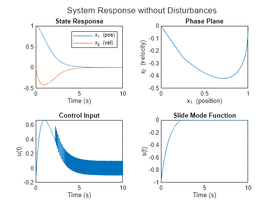
Phase Plane
The phase plane provides a visual representation of the system dynamics by plotting position versus velocity. In this plane, the system trajectory converges to the sliding surface, defined by the sliding function , which represents the desired system behavior. When the trajectory reaches the sliding surface, the system is in sliding mode and the controller guides it towards the target state.
Plot the phase plane, system trajectory, and sliding surface.
N = 20;
x1_values = linspace(-0.5,1.5, N);
x2_values = linspace(-1.0,1.0, N);
[X1,X2] = meshgrid(x1_values,x2_values);
XDOT = msdStateDer([],[X1(:), X2(:)].',u,param);

figure
hold on
quiver(X1(:),X2(:),XDOT(1,:).',XDOT(2,:).', ...
    MaxHeadSize=0.1, ...
    AutoScaleFactor=0.9);
plot(Y(:,1),Y(:,2))
plot([-0.5 1.5],-param.smc.c*[-0.5 1.5], ":")
xlim([min(X1(:)) max(X1(:))])
ylim([min(X2(:)) max(X2(:))])
xlabel("x1 (position)")
ylabel("x2 (velocity)")
title("Phase-Plane")
legend("df/dt","States","Slide Surface")

This plot shows a visual depiction of the mass-spring-damper system response and the influence of the sliding mode control.
Simulate System with Disturbances
In real-world scenarios, systems are often influenced by external disturbances that can affect their performance. To test the robustness of the SMC strategy, you can introduce a disturbance into the mass-spring-damper system simulation. The bounded disturbance is modeled as a time-varying function that directly affects the dynamics of the system, where .
For this example, consider a sinusoidal disturbance given by:
The SMC control law is designed to counteract the effects of disturbances and drive the system state towards the desired sliding surface. The control law is defined as:
where the term is an additional term that accounts for the upper bound of the disturbance. Define a handle to the disturbance function.
d = @(t) 0.5*sin(t);
Update the SMC controller parameters.
param.smc.c =5; param.smc.k =
3; param.smc.eta =
0.1; param.smc.d =
0.6;
Create a handle for the control input function and simulate the system response using ode45.
u = @(x,param) smc(x,param);
[T,Y] = ode45(@(t,x) msdStateDer(t,x,u,param,d),tspan,y0);
Calculate sliding surface, S, and control input values, U, over the simulation time.
S = -param.smc.c*Y(:,1) - Y(:,2);
U = smc(Y.',param);
Generate the plots to visualize the system response, phase plane, control input, and sliding surface over time.
plotResponse(T,U,Y,S,"System Response with Disturbances")
Reduce Chattering Using Quasi-Sliding Mode Control
A common issue in SMC is chattering, which is the high-frequency switching of the control input when the system state is close to the sliding surface. To mitigate chattering, quasi-sliding mode control can be employed. In this approach, the discontinuous sign function in the control law is replaced with a continuous approximation, such as a saturation function. [3]
For this example, use the following saturation function.
Here, is the boundary layer thickness. This saturation function smoothly interpolates between and when the sliding variable is within the boundary layer , which reduces the high-frequency switching.
The modified control law with the saturation function is given by:
The choice of is critical as it defines the thickness of the boundary layer around the sliding surface. A larger results in less chattering but can increase the steady-state error. Conversely, a smaller can reduce steady-state error but increase chattering.
To implement quasi-sliding mode control, define the saturation function using function handle sat and set the boundary layer thickness, , to 1e-2.
phi = 1e-2;
sat = @(s) min(max(s/phi,-1),1);
Update the control input function to include the saturation function.
u = @(x,param) smc(x,param,sat);
Simulate the system response using the updated control law.
[T,Y] = ode45(@(t,x) msdStateDer(t,x,u,param,d),tspan,y0);
Calculate the sliding surface and control input values over the simulation time.
S = -param.smc.c*Y(:,1) - Y(:,2);
U = smc(Y.',param,sat);
Visualize the system response, phase plane, control input, and sliding surface over time using QSMC.
plotResponse(T,U,Y,S,"System Response Using Quasi-Sliding Mode Control")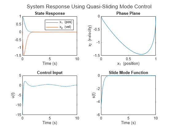
The quasi-sliding mode control system achieves similar performance with no chattering in the control input.
Simulink
In this section, design the SMC controller using the Sliding Mode Controller (Reaching Law) block in Simulink.
Open the Simulink® model.
mdl = 'massSpringDamper';
open_system(mdl)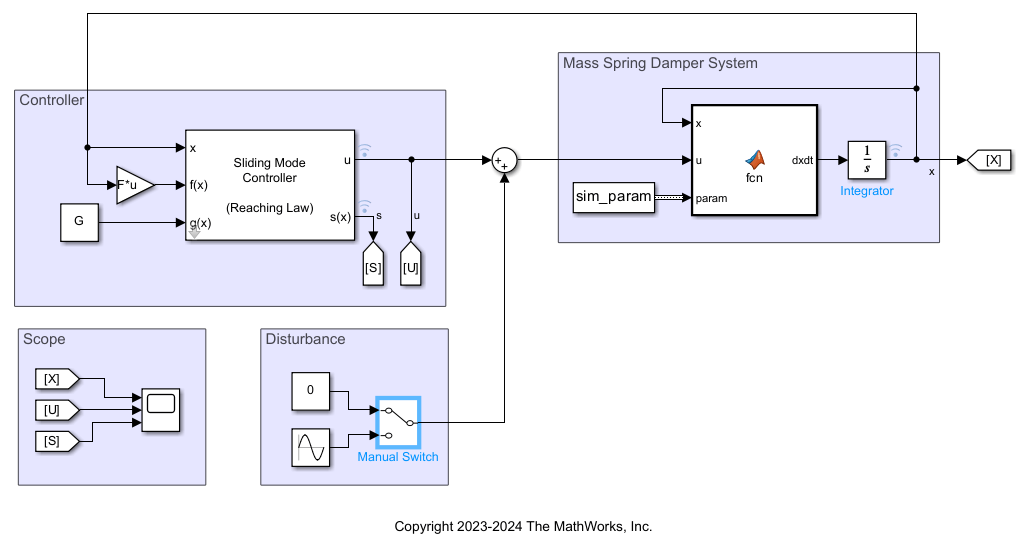
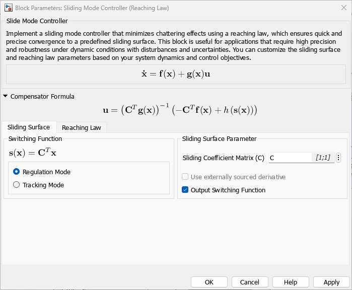
Open the Sliding Mode Controller (Reaching Law) block.
open_system(mdl+"/Sliding Mode Controller (Reaching Law)")
Note, the Sliding Mode Controller (Reaching Law) designs a controller for a dynamic system in the form of .
Define matrices F and G for the dynamic terms , and .
F = [0 1; -param.Stiffness/param.Mass -param.Damping/param.Mass];
G = [0; 1/param.Mass];
Specify the sliding coefficient matrix.
C = [1;1];
Specify the desired reaching law parameters using the 'Reaching Law' tab:
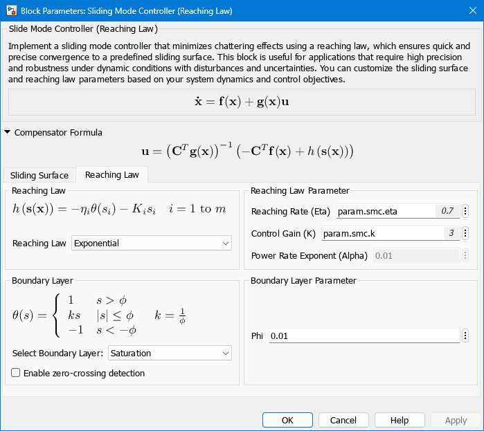
set_param([mdl '/Sliding Mode Controller (Reaching Law)'], 'BoundaryLayer', "Sign");
For this example, the Mass-Spring-Damper parameters are defined in the From Workspace block. Use the Simulink.Bus.createObject function to create the bus object, and update the From Workspace output data type accordingly.
sim_param = struct( ...
    'Mass', timeseries(param.Mass, 0), ...
    'Damping', timeseries(param.Damping, 0), ...
    'Stiffness', timeseries(param.Stiffness, 0));

busInfo = Simulink.Bus.createObject(param);
set_param([mdl '/From Workspace'], 'OutDataTypeStr', "Bus: " + busInfo.busName);
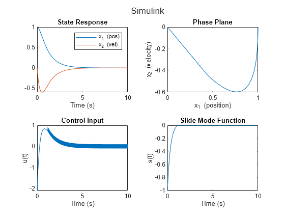
Simulate the model and view the results.
simout = sim(mdl);

T = simout.logsout.get('x').Values.Time;
U = squeeze(simout.logsout.get('u').Values.Data);
S = squeeze(simout.logsout.get('s').Values.Data);
Y = squeeze(simout.logsout.get('x').Values.Data).';

plotResponse(T,U,Y,S,"Simulink")

References
[1] Derbel, Nabil, Jawhar Ghommam, and Quanmin Zhu, eds. Applications of Sliding Mode Control. Vol. 79. Springer Singapore, 2017.
[2] Weibing Gao, and J.C. Hung. “Variable Structure Control of Nonlinear Systems: A New Approach.” IEEE Transactions on Industrial Electronics 40, no. 1 (February 1993): 45–55. https://doi.org/10.1109/41.184820.
[3] Richter, Hanz. Advanced control of turbofan engines. Springer Science & Business Media, 2011.
See Also
Sliding Mode Controller (Reaching Law)