Sliding Mode Control Design for a Robotic Manipulator
This example shows how to design a controller for a robotic manipulator with two actuated joints using sliding mode control (SMC). SMC is useful for systems that require robustness against disturbances and model uncertainties. Using SMC, you can obtain high-precision tracking of desired trajectories even in the presence of external disturbances and parameter variations. For more information on SMC, see Sliding Mode Control.
Dynamics of Robotic Manipulator
Consider the dynamics of a two-jointed robotic manipulator governed by the following dynamic equation.
Here:
, , and are 2-by-1 vectors representing the joint angles, velocities, and accelerations, respectively.
The control input is 2-by-1 torque vector applied to the joints.
The inertia matrix , Coriolis matrix , gravity vector , and friction vector encapsulate the dynamics of the manipulator
represents the disturbance torques affecting the system.
To facilitate control design, define the state variables and , and control input . Then define the more compact state-space representation of the system, .
The state vector is given by:
, where
Here, and
The robot manipulator dynamics are implemented in the robotStateFcn helper function. This function generates the state derivatives with respect to time based on the current state vector , the control input vector , and a vector of model parameters. For this example, assume that the friction model, is negligible and not used in calculations.
For this example, define the following parameters of the robot manipulator.
M = [0.5; 1.5]; % Masses of the first and second links (kg)
L = [1.0; 0.8]; % Lengths of the first and second link (m)
J = [5.0; 5.0]; % Moments of inertia of the first and second link (kgm^2)
Reference Trajectory for Robotic Manipulator
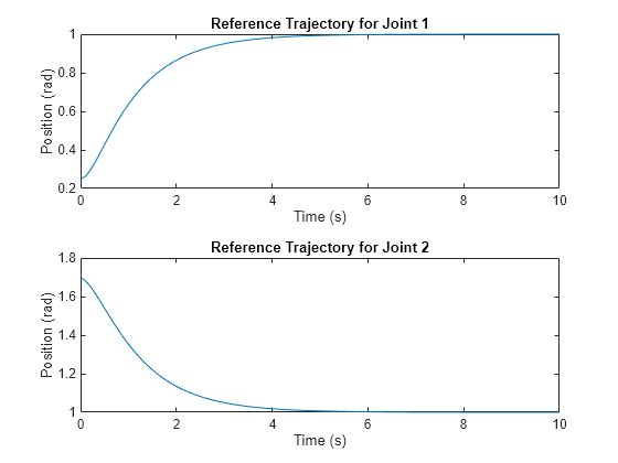
In this example, the reference trajectories for the two actuated joints of the robotic manipulator are described by time-varying exponential functions.
The reference trajectory primarily targets the set points , with additional terms ensuring a smooth transition from the initial position to these set points. The differentiation of these functions is essential for producing consistent velocity and acceleration profiles, contributing to the manipulators stability and precise movement. This characteristic also facilitates the use of control algorithms that require continuous and differentiable set points.
For this example, set the parameters for the reference trajectories of both joints. These parameters define the shape and behavior of the trajectory functions over time.
[a1,b1,c1,d1,e1] = deal(1,-1,0.25,-1,-4);
[a2,b2,c2,d2,e2] = deal(1,1,-0.3,-1,-3);
Plot the reference trajectories for both joints to visualize the target positions over the specified time interval.
qref = @(time,a,b,c,d,e) a + b*exp(d*time) + c*exp(e*time);
time = linspace(0,10);

figure
tiledlayout(2,1)

nexttile
plot(time,qref(time,a1,b1,c1,d1,e1))
title("Reference Trajectory for Joint 1")
ylabel("Position (rad)")
xlabel("Time (s)")

nexttile
plot(time,qref(time,a2,b2,c2,d2,e2))
title("Reference Trajectory for Joint 2")
ylabel("Position (rad)")
xlabel("Time (s)")
Design Sliding Mode Controller
SMC is a robust control strategy that forces the system state to converge to a predefined sliding surface and maintain this condition thereafter. This objective is achieved through the application of a discontinuous control action that switches depending on the system position relative to the sliding surface.
In this example, the SMC control law used is:
where:
correspond to the Exponential Reaching Law.
corresponds to the Boundary Layer Function.
corresponds to the Switching Function.
The control depends on the following parameters.
: Amplitude of the discontinuous control action, enhances robustness against disturbances.
: Proportional gain in the continuous part of the control law, reduces steady-state error and improves response time.
: Coefficient in the sliding surface, affects the rate of convergence to the sliding surface.
The terms and are dependent of the robot manipulator parameters. In real-world scenarios, you might not know these parameters exactly and only have estimated values available.
Here, the manipulator inertia matrix , Coriolis matrix , friction vector and gravity vector are estimated values.
For this example, define the following SMC controller parameters.
eta = [1; 3];           % Amplitude of discontinuous control action
K = [2; 1];             % Proportional gain
C = [5*eye(2); eye(2)]; % Sliding surface coefficient
Phi = 0.01;             % Boundary layer thickness
Closed-Loop Simulation Using SMC Controller
To evaluate the performance of the designed SMC controller, simulate the robotic manipulator in Simulink®. The simulation tests the controller reference tracking under conditions of both known and uncertain parameters.
Open the model.
mdl = "robotManipulatorModel";
open_system(mdl)
Simulate the system starting from any initial position with zero velocity using the signum function.
Define the initial state of the robotic manipulator.
x0 = [0;0;0;0];
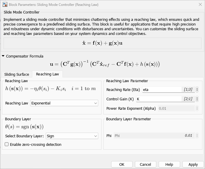
Choose the variant of the reaching law and boundary layer. In this case, use the Exponential reaching law and the sign function for boundary layer.
set_param(mdl+"/Sliding Mode Controller (Reaching Law)", "ReachingLaw", "Exponential");
set_param(mdl+"/Sliding Mode Controller (Reaching Law)", "BoundaryLayer", "Sign");
Set the robot dynamics parameters for the simulation within the Estimator subsystem, assuming that the robot parameters are known and unaffected by any external disturbances.
[Md,Ld,Jd] = deal(M,L,J);
Simulate the model.
simout = sim(mdl);
Post process the simulation results for plotting.
[sim1, ref] = postProcessSimResults(simout);
Simulate the system with the same initial conditions but with a parameter mismatch between the robot and the Estimator subsystem. Doing so tests the robustness of the SMC controller against model uncertainties.
Md = [0.1; 1.0];
Ld = [1.0; 0.8];
Jd = [4.0; 6.0];

simout = sim(mdl);
sim2 = postProcessSimResults(simout);
Plot the simulation results.
figure
stackedplot(ref,sim1,sim2, ["q1","q2","qdot1","qdot2"], Title="State Trajectories");
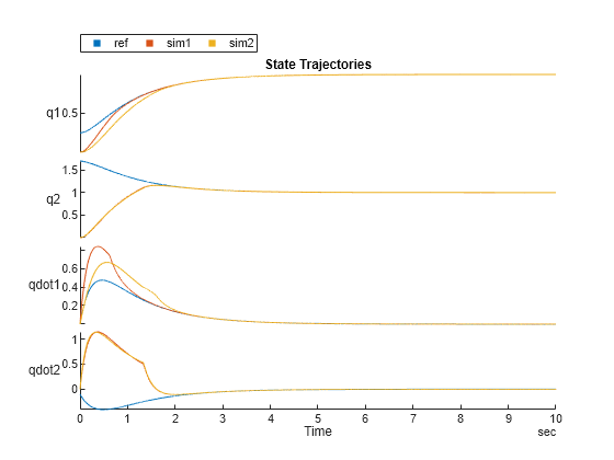
The SMC controller is still capable of tracking the reference trajectory even after adjusting the parameters.
Visualize the controller performance by plotting the control inputs and the sliding mode function.
figure
stackedplot(sim1,sim2, {"Tau1","S1","Tau2","S2"}, Title="Control Inputs and Slide Mode Function Plots");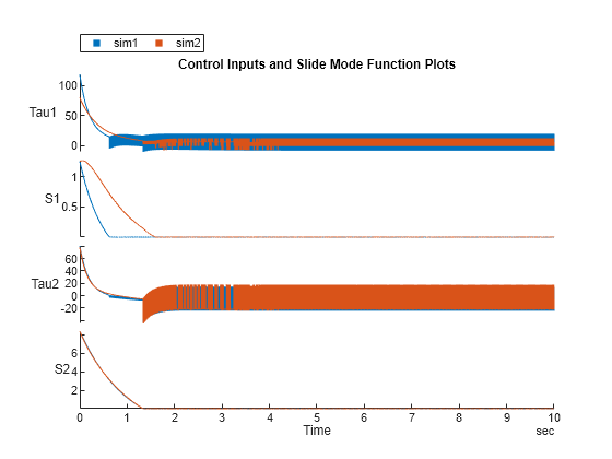
Reduce Control Input Chattering
Due to the use of the signum function in the SMC controller, the control input exhibits chattering. One common practice to reduce chattering is to use the saturation function instead of the sign function.
% switch the controller to use saturation function
set_param(mdl+"/Sliding Mode Controller (Reaching Law)", "BoundaryLayer", "Saturation");
Assign known dynamic parameters to the controller for the first simulation run.
[Md,Ld,Jd] = deal(M,L,J);
Execute the simulation with the saturation function in place.
simout = sim(mdl);
[sim3, ref] = postProcessSimResults(simout);
Specify the mismatched parameter values and simulate the robot.
Md = [0.1; 1.0];
Ld = [1.0; 0.8];
Jd = [4.0; 6.0];

simout = sim(mdl);
sim4 = postProcessSimResults(simout);
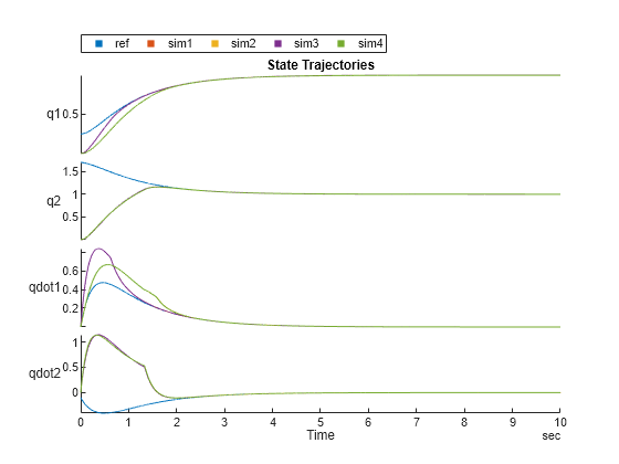
Plot the state trajectories to compare the performance of the controller with the saturation function against the reference trajectories and previous results.
figure
stackedplot(ref,sim1,sim2,sim3,sim4, ["q1","q2","qdot1","qdot2"], Title="State Trajectories")
Plot the control inputs and sliding mode function.
figure
stackedplot(sim3,sim4, {"Tau1","S1","Tau2","S2"}, Title="Control Inputs and Slide Mode Function Plots");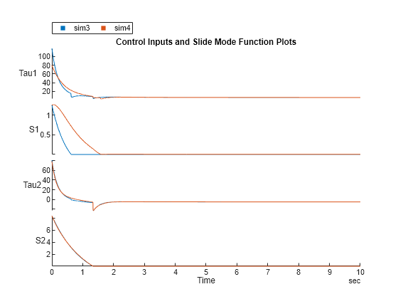
When you use the saturation function in the control law, chattering is significantly reduced in the control input.
Another way to reduce chattering is to use the relay function instead of the sign function. You can try it out by selecting "relay" in the variant subsystem in the Simulink model.
See Also
Sliding Mode Controller (Reaching Law)