plot
Description
plot( plots the measured and simulated
impedances for all profiles inside the eisfom)EISModel object,
eisfom.
plot(___, also
specifies options using one or more name-value arguments.Name=Value)
chart = plot(___)ImpedanceVerificationChart object.
Examples
This example shows how to plot the measured and simulated impedance
for all profiles inside an EISModel object.
Open the DownloadBatteryEISData example and load the required
electrochemical impedance spectroscopy (EIS) data. This data has been generated from a
battery with a nominal capacity of 30/1000 A*Hr at a temperature of
25 °C. This data consists of a 500-by-3 matrix of
doubles. The columns of the matrix refer to the frequency, real impedance, and imaginary
impedance values, respectively.
openExample("simscapebattery/DownloadBatteryEISDataExample")
load("generatedEISData.mat")
Fit the EIS data to a fractional-order equivalent circuit model. To fit the data and
create an EISModel object, use the fitEISModel
function.
eisfom = fitEISModel(eisData);
Analyze how the function performed the fit on the frequency model by using the
plot function. This plot shows the simulated data against the
measured data, where the X-axis represents the real part of the
impedance and the Y-axis represents the imaginary part of the
impedance.
plot(eisfom,Parent=figure,DisplayMode="Nyquist")
You can also plot the imaginary impedance over the log frequency by setting the
DisplayMode argument to "ImagZ(f)".
plot(eisfom,Parent=figure,DisplayMode="ImagZ(f)")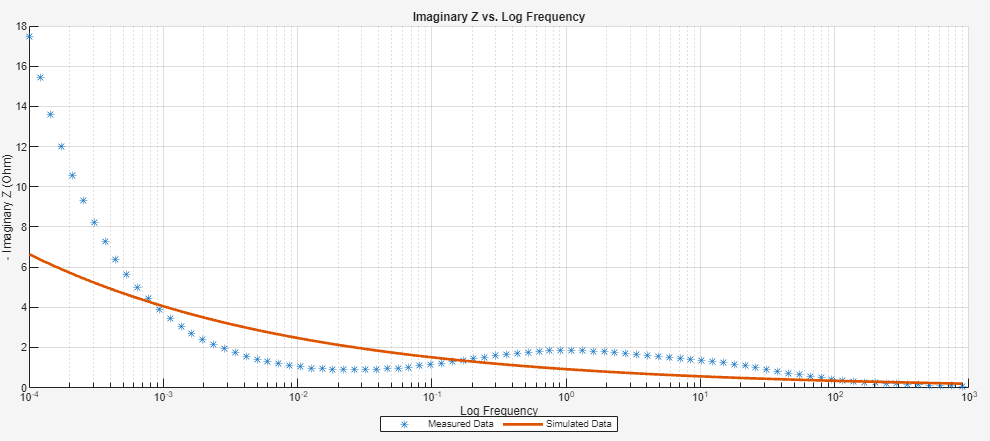
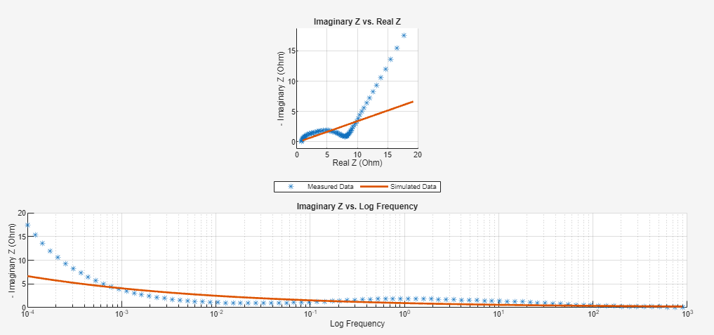
To plot both figures, set the DisplayMode argument to
"Nyq_ImagZ(f)".
Input Arguments
Name-Value Arguments
Specify optional pairs of arguments as
Name1=Value1,...,NameN=ValueN, where Name is
the argument name and Value is the corresponding value.
Name-value arguments must appear after other arguments, but the order of the
pairs does not matter.
Example: plotPulse(myTest,indices,PlottingQuadrant="fourth")
Plot Arguments
ComponentContainer Arguments
Background color, specified as an RGB triplet, a hexadecimal color code, or one of the color options listed in the table.
RGB triplets and hexadecimal color codes are useful for specifying custom colors.
An RGB triplet is a three-element row vector whose elements specify the intensities of the red, green, and blue components of the color. The intensities must be in the range
[0,1]; for example,[0.4 0.6 0.7].A hexadecimal color code is a character vector or a string scalar that starts with a hash symbol (
#) followed by three or six hexadecimal digits, which can range from0toF. The values are not case sensitive. Thus, the color codes"#FF8800","#ff8800","#F80", and"#f80"are equivalent.
Alternatively, you can specify some common colors by name. This table lists the named color options, the equivalent RGB triplets, and hexadecimal color codes.
| Color Name | Short Name | RGB Triplet | Hexadecimal Color Code | Appearance |
|---|---|---|---|---|
"red" | "r" | [1 0 0] | "#FF0000" |
|
"green" | "g" | [0 1 0] | "#00FF00" |
|
"blue" | "b" | [0 0 1] | "#0000FF" |
|
"cyan"
| "c" | [0 1 1] | "#00FFFF" |
|
"magenta" | "m" | [1 0 1] | "#FF00FF" |
|
"yellow" | "y" | [1 1 0] | "#FFFF00" |
|
"black" | "k" | [0 0 0] | "#000000" |
|
"white" | "w" | [1 1 1] | "#FFFFFF" |
|
Here are the RGB triplets and hexadecimal color codes for the default colors MATLAB uses in many types of plots.
| RGB Triplet | Hexadecimal Color Code | Appearance |
|---|---|---|
[0 0.4470 0.7410] | "#0072BD" |
|
[0.8500 0.3250 0.0980] | "#D95319" |
|
[0.9290 0.6940 0.1250] | "#EDB120" |
|
[0.4940 0.1840 0.5560] | "#7E2F8E" |
|
[0.4660 0.6740 0.1880] | "#77AC30" |
|
[0.3010 0.7450 0.9330] | "#4DBEEE" |
|
[0.6350 0.0780 0.1840] | "#A2142F" |
|
State of visibility, specified as 'on' or
'off', or as numeric or logical 1
(true) or 0 (false). A
value of 'on' is equivalent to true, and
'off' is equivalent to false. Thus, you can
use the value of this property as a logical value. The value is stored as an on/off
logical value of type matlab.lang.OnOffSwitchState.
'on'— Display the object.'off'— Hide the object without deleting it. You still can access the properties of an invisible UI component.
To make your app start faster, set the Visible property to
'off' for all components that do not need to appear at
startup.
Changing the size of an invisible container triggers the
SizeChangedFcn callback when it becomes visible.
Changing the Visible property of a container does
not change the values of the Visible
properties of child components. This is true even though hiding the container causes
the child components to be hidden.
Context menu, specified as a ContextMenu object created using
the uicontextmenu function. Use this
property to display a context menu when you right-click on an area of the component
that does not contain any underlying UI components or graphics objects.
To display a context menu when you right-click on any portion of the custom UI
component, write code to set the ContextMenu property of all
underlying UI components and graphics objects whenever the
ContextMenu property of your custom component is set.
Example: Component With Context Menu
This code creates a simple custom UI component with a label and a button in a
grid layout manager. Whenever a user creates an instance of the
SimpleComponent class and assigns a context menu to the
component, the code in the update method then assigns that same
context menu to the underlying GridLayout,
Button, and Label objects.
classdef SimpleComponent < matlab.ui.componentcontainer.ComponentContainer

    properties (Access = private, Transient, NonCopyable)
        GridLayout matlab.ui.container.GridLayout
        Button matlab.ui.control.Button
        Label matlab.ui.control.Label
    end

    methods (Access=protected)
        function setup(obj)
            % Set component size
            obj.Position = [100 100 220 50];
            % Create grid
            obj.GridLayout = uigridlayout(obj,[1 2]);
            % Create components
            obj.Label = uilabel(obj.GridLayout,...
                "Text","My component");
            obj.Button = uibutton(obj.GridLayout);
        end

        function update(obj)
            obj.GridLayout.ContextMenu = obj.ContextMenu;
            obj.Label.ContextMenu = obj.ContextMenu;
            obj.Button.ContextMenu = obj.ContextMenu;
        end
    end
end
Create a SimpleComponent object and specify a context menu.
Right-click on the empty space in the component and on the label. The context menu
appears.
fig = uifigure;
cm = uicontextmenu(fig);
m1 = uimenu(cm);
SimpleComponent(fig,"ContextMenu",cm);UI component size and location, excluding the margins for decorations such as axis
labels and tick marks. Specify this property as a vector of form [left bottom
width height].
Note
Setting this property has no effect when the parent of the UI component is a
GridLayout.
Units of measurement, specified as 'normalized',
'centimeters', 'pixels'
,'characters', 'points', or
'inches'.
Layout options, specified as a GridLayoutOptions object. This
property specifies options for components that are children of grid layout containers.
If the component is not a child of a grid layout container (for example, it is a child
of a figure or panel), then this property is empty and has no effect. However, if the
component is a child of a grid layout container, you can place the component in the
intended row and column of the grid by setting the Row and
Column properties of the GridLayoutOptions
object.
For example, this code places an image component in the third row and second column of its parent grid.
g = uigridlayout([4 3]);
im = uiimage(g);
im.ImageSource = 'peppers.png';
im.ScaleMethod = 'fill';
im.Layout.Row = 3;
im.Layout.Column = 2;
To make the image span multiple rows or columns, specify the
Row or Column property as a two-element
vector. For example, this image spans columns 2 through
3.
im.Layout.Column = [2 3];
Size change callback, specified as one of these values:
A function handle.
A cell array in which the first element is a function handle. Subsequent elements in the cell array are the arguments to pass to the callback function.
A character vector containing a valid MATLAB® expression (not recommended). MATLAB evaluates this expression in the base workspace.
The SizeChangedFcn callback executes when:
The component becomes visible for the first time.
The component is visible while its size changes.
This component becomes visible for the first time after its size changes. This situation occurs when the size changes while the component is invisible, and then it becomes visible later.
Object creation function, specified as one of these values:
Function handle.
Cell array in which the first element is a function handle. Subsequent elements in the cell array are the arguments to pass to the callback function.
Character vector containing a valid MATLAB expression (not recommended). MATLAB evaluates this expression in the base workspace.
For more information about specifying a callback as a function handle, cell array, or character vector, see Callbacks in App Designer.
This property specifies a callback function to execute when MATLAB creates the object. MATLAB initializes all property values before executing the
CreateFcn callback. If you do not specify the
CreateFcn property, then MATLAB executes a default creation function.
Setting the CreateFcn property on an existing component has
no effect.
If you specify this property as a function handle or cell array, you can access
the object that is being created using the first argument of the callback function.
Otherwise, use the gcbo function to access the
object.
Object deletion function, specified as one of these values:
Function handle.
Cell array in which the first element is a function handle. Subsequent elements in the cell array are the arguments to pass to the callback function.
Character vector containing a valid MATLAB expression (not recommended). MATLAB evaluates this expression in the base workspace.
For more information about specifying a callback as a function handle, cell array, or character vector, see Callbacks in App Designer.
This property specifies a callback function to execute when MATLAB deletes the object. MATLAB executes the DeleteFcn callback before destroying
the properties of the object. If you do not specify the DeleteFcn
property, then MATLAB executes a default deletion function.
If you specify this property as a function handle or cell array, you can access
the object that is being deleted using the first argument of the callback function.
Otherwise, use the gcbo function to access the
object.
Callback interruption, specified as 'on' or
'off', or as numeric or logical 1
(true) or 0 (false). A
value of 'on' is equivalent to true, and
'off' is equivalent to false. Thus, you can
use the value of this property as a logical value. The value is stored as an on/off
logical value of type matlab.lang.OnOffSwitchState.
This property determines if a running callback can be interrupted. There are two callback states to consider:
The running callback is the currently executing callback.
The interrupting callback is a callback that tries to interrupt the running callback.
Whenever MATLAB invokes a callback, that callback attempts to interrupt the running
callback (if one exists). The Interruptible property of the
object owning the running callback determines if interruption is allowed.
A value of
'on'allows other callbacks to interrupt the object's callbacks. The interruption occurs at the next point where MATLAB processes the queue, such as when there is adrawnow,figure,uifigure,getframe,waitfor, orpausecommand.If the running callback contains one of those commands, then MATLAB stops the execution of the callback at that point and executes the interrupting callback. MATLAB resumes executing the running callback when the interrupting callback completes.
If the running callback does not contain one of those commands, then MATLAB finishes executing the callback without interruption.
A value of
'off'blocks all interruption attempts. TheBusyActionproperty of the object owning the interrupting callback determines if the interrupting callback is discarded or put into a queue.
Note
Callback interruption and execution behave differently in these situations:
If the interrupting callback is a
DeleteFcn,CloseRequestFcnorSizeChangedFcncallback, then the interruption occurs regardless of theInterruptibleproperty value.If the running callback is currently executing the
waitforfunction, then the interruption occurs regardless of theInterruptibleproperty value.Timerobjects execute according to schedule regardless of theInterruptibleproperty value.
When an interruption occurs, MATLAB does not save the state of properties or the display. For example, the
object returned by the gca or gcf command might change when another callback executes.
Callback queuing, specified as 'queue' or
'cancel'. The BusyAction property determines
how MATLAB handles the execution of interrupting callbacks. There are two callback
states to consider:
The running callback is the currently executing callback.
The interrupting callback is a callback that tries to interrupt the running callback.
Whenever MATLAB invokes a callback, that callback attempts to interrupt a running
callback. The Interruptible property of the object owning the
running callback determines if interruption is permitted. If interruption is not
permitted, then the BusyAction property of the object owning the
interrupting callback determines if it is discarded or put in the queue. These are
possible values of the BusyAction property:
'queue'— Puts the interrupting callback in a queue to be processed after the running callback finishes execution.'cancel'— Does not execute the interrupting callback.
Deletion status, returned as an on/off logical value of type matlab.lang.OnOffSwitchState.
MATLAB sets the BeingDeleted property to
'on' when the DeleteFcn callback begins
execution. The BeingDeleted property remains set to
'on' until the component object no longer exists.
Check the value of the BeingDeleted property to verify that
the object is not about to be deleted before querying or modifying it.
Parent container of the component, specified as a Figure,
Panel, Tab, or GridLayout
object.
UI component children, returned as an empty GraphicsPlaceholder
array. Custom UI components have no children. Setting this property has no
effect.
Visibility of the object handle, specified as 'on',
'callback', or 'off'.
This property controls the visibility of the object in its parent's list of
children. When an object is not visible in its parent's list of children, it is not
returned by functions that obtain objects by searching the object hierarchy or
querying properties. These functions include get, findobj, clf, and close. Objects are valid even if they are
not visible. If you can access an object, you can set and get its properties, and pass
it to any function that operates on objects.
| HandleVisibility Value | Description |
|---|---|
'on' | The object is always visible. |
'callback' | The object is visible from within callbacks or functions invoked by callbacks, but not from within functions invoked from the command line. This option blocks access to the object at the command-line, but allows callback functions to access it. |
'off' | The object is invisible at all times. This option is useful for
preventing unintended changes to the UI by another function. Set the
HandleVisibility to 'off' to
temporarily hide the object during the execution of that function. |
Type of UI component object, returned as character vector containing the component name.
Object identifier, specified as a character
vector or string scalar. You can specify a unique Tag value to
serve as an identifier for an object. When you need access to the object elsewhere in
your code, you can use the findobj function to search for the object
based on the Tag value.
User data, specified as any MATLAB array. For example, you can specify a scalar, vector, matrix, cell array, character array, table, or structure. Use this property to store arbitrary data on an object.
If you are working in App Designer, create public or private properties in the app
to share data instead of using the UserData property. For more
information, see Share Data Within a Single App Designer App.
Output Arguments
Version History
Introduced in R2025a