Take Derivatives of a Signal
You want to differentiate a signal without increasing the noise power. MATLAB®'s function diff amplifies the noise, and the resulting inaccuracy worsens for higher derivatives. To fix this problem, use a differentiator filter instead.
Analyze the displacement of a building floor during an earthquake. Find the speed and acceleration as functions of time.
Load the file earthquake. The file contains the following variables:
drift: Floor displacement, measured in centimeterst: Time, measured in secondsFs: Sample rate, equal to 1 kHz
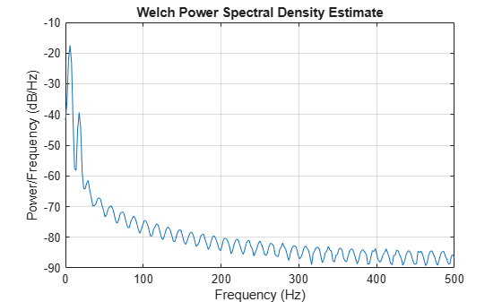
load('earthquake.mat')Use pwelch to display an estimate of the power spectrum of the signal. Note how most of the signal energy is contained in frequencies below 100 Hz.
pwelch(drift,[],[],[],Fs)
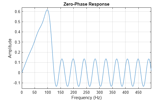
Use designfilt to design an FIR differentiator of order 50. To include most of the signal energy, specify a passband frequency of 100 Hz and a stopband frequency of 120 Hz. Inspect the filter with zerophase.
Nf = 50;
Fpass = 100;
Fstop = 120;

d = designfilt('differentiatorfir','FilterOrder',Nf, ...
    'PassbandFrequency',Fpass,'StopbandFrequency',Fstop, ...
    'SampleRate',Fs);

zerophase(d,[],Fs)
Differentiate the drift to find the speed. Divide the derivative by dt, the time interval between consecutive samples, to set the correct units.
dt = t(2)-t(1);

vdrift = filter(d,drift)/dt;
The filtered signal is delayed. Use grpdelay to determine that the delay is half the filter order. Compensate for it by discarding samples.
delay = mean(grpdelay(d))
delay =
25
tt = t(1:end-delay);
vd = vdrift;
vd(1:delay) = [];
The output also includes a transient whose length equals the filter order, or twice the group delay. delay samples were discarded above. Discard delay more to eliminate the transient.
tt(1:delay) = [];
vd(1:delay) = [];
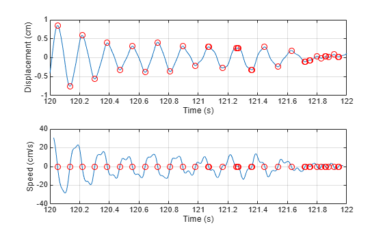
Plot the drift and the drift speed. Use findpeaks to verify that the maxima and minima of the drift correspond to the zero crossings of its derivative.
[pkp,lcp] = findpeaks(drift);
zcp = zeros(size(lcp));

[pkm,lcm] = findpeaks(-drift);
zcm = zeros(size(lcm));

subplot(2,1,1)
plot(t,drift,t([lcp lcm]),[pkp -pkm],'or')
xlabel('Time (s)')
ylabel('Displacement (cm)')
grid

subplot(2,1,2)
plot(tt,vd,t([lcp lcm]),[zcp zcm],'or')
xlabel('Time (s)')
ylabel('Speed (cm/s)')
grid
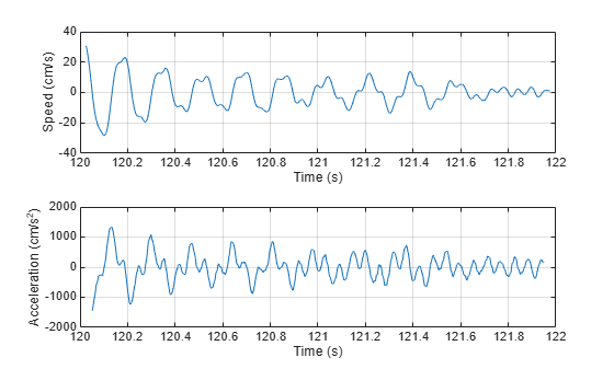
Differentiate the drift speed to find the acceleration. The lag is twice as long. Discard twice as many samples to compensate for the delay, and the same number to eliminate the transient. Plot the speed and acceleration.
adrift = filter(d,vdrift)/dt;

at = t(1:end-2*delay);
ad = adrift;
ad(1:2*delay) = [];

at(1:2*delay) = [];
ad(1:2*delay) = [];

subplot(2,1,1)
plot(tt,vd)
xlabel('Time (s)')
ylabel('Speed (cm/s)')
grid

subplot(2,1,2)
plot(at,ad)
ax = gca;
ax.YLim = 2000*[-1 1];
xlabel('Time (s)')
ylabel('Acceleration (cm/s^2)')
grid
Compute the acceleration using diff. Add zeros to compensate for the change in array size. Compare the result to that obtained with the filter. Notice the amount of high-frequency noise.
vdiff = diff([drift;0])/dt;
adiff = diff([vdiff;0])/dt;

subplot(2,1,1)
plot(at,ad)
ax = gca;
ax.YLim = 2000*[-1 1];
xlabel('Time (s)')
ylabel('Acceleration (cm/s^2)')
grid
legend('Filter')
title('Acceleration with Differentiation Filter')

subplot(2,1,2)
plot(t,adiff)
ax = gca;
ax.YLim = 2000*[-1 1];
xlabel('Time (s)')
ylabel('Acceleration (cm/s^2)')
grid
legend('diff')

See Also
findpeaks | designfilt | grpdelay | periodogram | zerophase