pulstran
Pulse train
Description
Examples
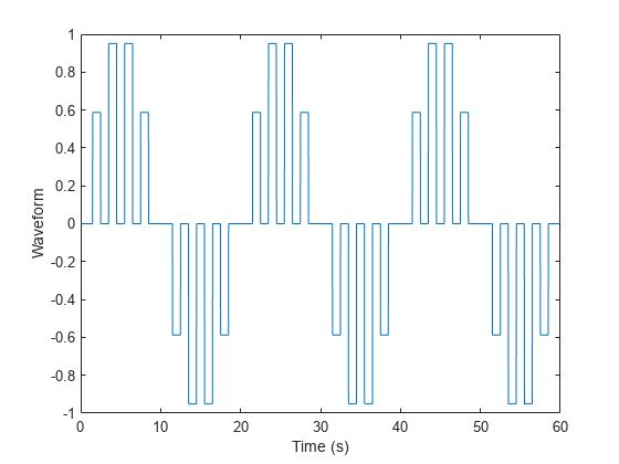
This example generates a pulse train using the default rectangular pulse of unit width. The repetition frequency is 0.5 Hz, the signal length is 60 s, and the sample rate is 1 kHz. The gain factor is a sinusoid of frequency 0.05 Hz.
t = 0:1/1e3:60;
d = [0:2:60;sin(2*pi*0.05*(0:2:60))]';
x = @rectpuls;
y = pulstran(t,d,x);

plot(t,y)
hold off
xlabel('Time (s)')
ylabel('Waveform')
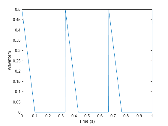
This example generates an asymmetric sawtooth waveform with a repetition frequency of 3 Hz. The sawtooth has width 0.2 s and skew factor –1. The signal length is 1 s, and the sample rate is 1 kHz. Plot the pulse train.
fs = 1e3;
t = 0:1/1e3:1;
d = 0:1/3:1;
x = tripuls(t,0.2,-1);
y = pulstran(t,d,x,fs);

plot(t,y)
hold off
xlabel('Time (s)')
ylabel('Waveform')
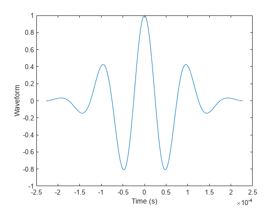
Plot a 10 kHz Gaussian RF pulse with 50% bandwidth, sampled at a rate of 10 MHz. Truncate the pulse where the envelope falls 40 dB below the peak.
fs = 1e7;
tc = gauspuls('cutoff',10e3,0.5,[],-40);
t = -tc:1/fs:tc;
x = gauspuls(t,10e3,0.5);

plot(t,x)
xlabel('Time (s)')
ylabel('Waveform')
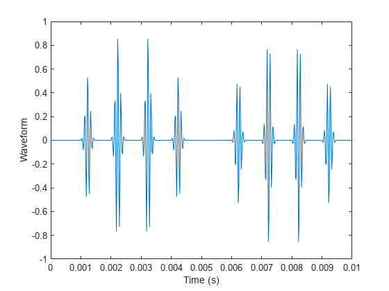
The pulse repetition frequency is 1 kHz, the sample rate is 50 kHz, and the pulse train length is 25 ms. The gain factor is a sinusoid of frequency 0.1 Hz.
ts = 0:1/50e3:0.025;
d = [0:1/1e3:0.025;sin(2*pi*0.1*(0:25))]';
y = pulstran(ts,d,x,fs);
Plot the periodic Gaussian pulse train.
plot(ts,y)
xlim([0 0.01])
xlabel('Time (s)')
ylabel('Waveform')
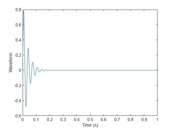
Write a function that generates custom pulses consisting of a sinusoid damped by an exponential. The pulse is an odd function of time. The generating function has a second input argument that specifies a single value for the sinusoid frequency and the damping factor. Display a generated pulse, sampled at 1 kHz for 1 second, with a frequency and damping value, both equal to 30.
fnx = @(x,fn) sin(2*pi*fn*x).*exp(-fn*abs(x));

ffs = 1000;
tp = 0:1/ffs:1;

pp = fnx(tp,30);

plot(tp,pp)
xlabel('Time (s)')
ylabel('Waveform')
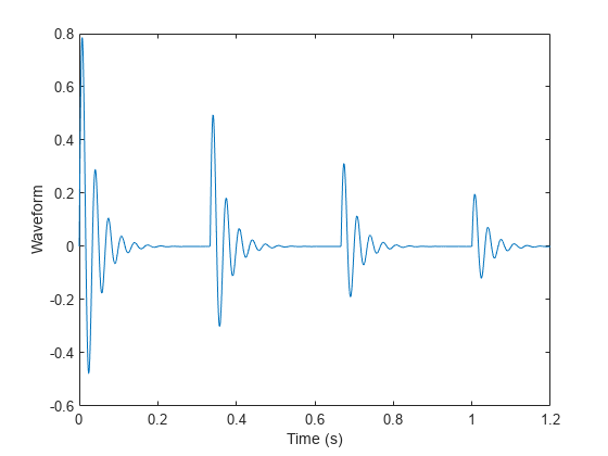
Use the pulstran function to generate a train of custom pulses. The train is sampled at 2 kHz for 1.2 seconds. The pulses occur every third of a second and have exponentially decreasing amplitudes.
Initially specify the generated pulse as a prototype. Include the prototype sample rate in the function call. In this case, pulstran replicates the pulses at the specified locations.
fs = 2e3;
t = 0:1/fs:1.2;

d = 0:1/3:1;
dd = [d;4.^-d]';

z = pulstran(t,dd,pp,ffs);

plot(t,z)
xlabel('Time (s)')
ylabel('Waveform')
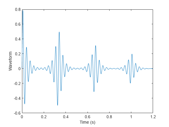
Generate the pulse train again, but now use the generating function as an input argument. Include the frequency and damping parameter in the function call. In this case, pulstran generates the pulse so that it is centered about zero.
y = pulstran(t,dd,fnx,30);

plot(t,y)
xlabel('Time (s)')
ylabel('Waveform')
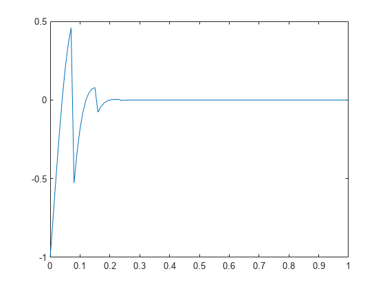
Write a function that generates a custom exponentially decaying sawtooth waveform of frequency 0.25 Hz. The generating function has a second input argument that specifies a single value for the sawtooth frequency and the damping factor. Display a generated pulse, sampled at 0.1 kHz for 1 second, with a frequency and damping value equal to 50.
fnx = @(x,fn) sawtooth(2*pi*fn*0.25*x).*exp(-2*fn*x.^2);

fs = 100;
t = 0:1/fs:1;

pp = fnx(t,50);

plot(t,pp)
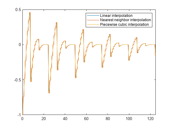
Use the pulstran function to generate a train of custom pulses. The train is sampled at 0.1 kHz for 125 seconds. The pulses occur every 25 seconds and have exponentially decreasing amplitudes.
Specify the generated pulse as a prototype. Generate three pulse trains using the default linear interpolation method, nearest neighbor interpolation and piecewise cubic interpolation. Compare the pulse trains on a single plot.
d = [0:25:125; exp(-0.015*(0:25:125))]';
ffs = 100;
tp = 0:1/ffs:125;

r = pulstran(tp,d,pp);
y = pulstran(tp,d,pp,"nearest");
q = pulstran(tp,d,pp,"pchip");


plot(tp,r)
hold on
plot(tp,y)
plot(tp,q)
xlim([0 125])
legend(["Linear" "Nearest neighbor" "Piecewise cubic"]+" interpolation")
hold off
Input Arguments
Time values at which func is evaluated, specified as a
vector.
Offset removed from the values of the array t, specified as a
real vector. You can apply an optional gain factor to each delayed evaluation by
specifying d as a two-column matrix, with offset defined in column
1 and associated gain in column 2. If you specify d as a row
vector, the values are interpreted as delays only.
Continuous function used to generate a pulse train based on its samples, specified
as 'rectpuls', 'gauspuls',
'tripuls', or a function handle.
If you use func as a function handle, you can pass the function
parameters as follows:
y = pulstran(t,d,'gauspuls',10e3,0.5);
This creates a pulse train using a 10 kHz Gaussian pulse with 50% bandwidth.
Prototype function, specified as a vector. The interval of p is
given by [0,(length(p)-1)/fs], and its samples are identically zero
outside this interval. By default, linear interpolation is used for generating
delays.
Sample rate in Hz, specified as a real scalar.
Interpolation method, specified as one of the options in this table.
Method | Description | Continuity | Comments |
|---|---|---|---|
| Linear interpolation. The interpolated value at a query point is based on linear interpolation of the values at neighboring grid points in each respective dimension. This is the default interpolation method. | C0 |
|
| Nearest neighbor interpolation. The interpolated value at a query point is the value at the nearest sample grid point. | Discontinuous |
|
| Next neighbor interpolation. The interpolated value at a query point is the value at the next sample grid point. | Discontinuous |
|
| Previous neighbor interpolation. The interpolated value at a query point is the value at the previous sample grid point. | Discontinuous |
|
| Shape-preserving piecewise cubic interpolation. The interpolated value at a query point is based on a shape-preserving piecewise cubic interpolation of the values at neighboring grid points. | C1 |
|
| Cubic convolution used in MATLAB® 5. | C1 | Points must be uniformly spaced. |
| Modified Akima cubic Hermite interpolation. The interpolated value at a query point is based on a piecewise function of polynomials with a degree of at most three. The Akima formula is modified to avoid overshoots. | C1 |
|
| Spline interpolation using not-a-knot end conditions. The interpolated value at a query point is based on a cubic interpolation of the values at neighboring grid points in each respective dimension. | C2 |
|
Output Arguments
Pulse train generated by the function, returned as a vector.
Extended Capabilities
Refer to the usage notes and limitations in the C/C++ Code Generation section. The same usage notes and limitations apply to GPU code generation.
Version History
Introduced before R2006a
MATLAB Command
You clicked a link that corresponds to this MATLAB command:
Run the command by entering it in the MATLAB Command Window. Web browsers do not support MATLAB commands.
Select a Web Site
Choose a web site to get translated content where available and see local events and offers. Based on your location, we recommend that you select: .
You can also select a web site from the following list
How to Get Best Site Performance
Select the China site (in Chinese or English) for best site performance. Other MathWorks country sites are not optimized for visits from your location.
Americas
- América Latina (Español)
- Canada (English)
- United States (English)
Europe
- Belgium (English)
- Denmark (English)
- Deutschland (Deutsch)
- España (Español)
- Finland (English)
- France (Français)
- Ireland (English)
- Italia (Italiano)
- Luxembourg (English)
- Netherlands (English)
- Norway (English)
- Österreich (Deutsch)
- Portugal (English)
- Sweden (English)
- Switzerland
- United Kingdom (English)