hht
Hilbert-Huang transform
Syntax
Description
hs = hht(IMFs)hs of the signal specified by
intrinsic mode functions IMFs. hs is
useful for analyzing signals that comprise a mixture of signals whose spectral
content changes in time. Use hht to perform Hilbert
spectral analysis on signals to identify localized features.
[___] = hht(___,
estimates Hilbert spectrum parameters with additional options specified by one
or more name-value arguments.Name=Value)
hht(___) with no output arguments plots the
Hilbert spectrum in the current figure window. You can use this syntax with any
of the input arguments in previous syntaxes.
hht(___,
plots the Hilbert spectrum with the optional freqlocation)freqlocation
argument to specify the location of the frequency axis. Frequency is represented
on the y-axis by default.
Examples
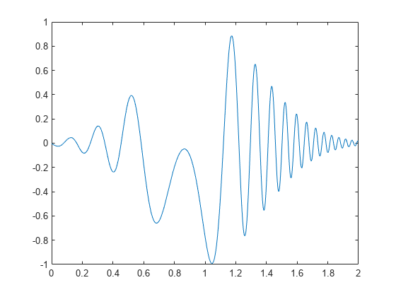
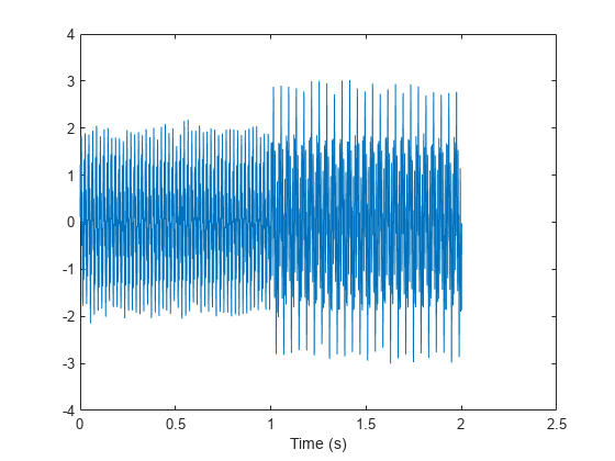
Generate a Gaussian-modulated quadratic chirp. Specify a sample rate of 2 kHz and a signal duration of 2 seconds.
fs = 2000;
t = 0:1/fs:2-1/fs;
q = chirp(t-2,4,1/2,6,'quadratic',100,'convex').*exp(-4*(t-1).^2);
plot(t,q)
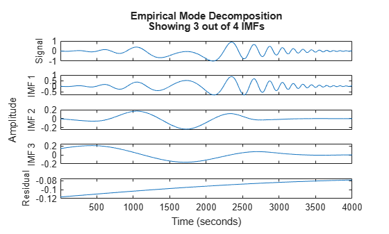
Use emd to visualize the intrinsic mode functions (IMFs) and the residual.
emd(q)
Compute the IMFs of the signal. Use the 'Display' name-value pair to output a table showing the number of sifting iterations, the relative tolerance, and the sifting stop criterion for each IMF.
imf = emd(q,'Display',1);Current IMF | #Sift Iter | Relative Tol | Stop Criterion Hit
1 | 2 | 0.0063952 | SiftMaxRelativeTolerance
2 | 2 | 0.1007 | SiftMaxRelativeTolerance
3 | 2 | 0.01189 | SiftMaxRelativeTolerance
4 | 2 | 0.0075124 | SiftMaxRelativeTolerance
Decomposition stopped because the number of extrema in the residual signal is less than the 'MaxNumExtrema' value.
Use the computed IMFs to plot the Hilbert spectrum of the quadratic chirp. Restrict the frequency range from 0 Hz to 20 Hz.
hht(imf,fs,'FrequencyLimits',[0 20])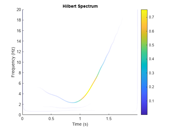
Load and visualize a nonstationary continuous signal composed of sinusoidal waves with a distinct change in frequency. The vibration of a jackhammer and the sound of fireworks are examples of nonstationary continuous signals. The signal is sampled at a rate fs.
load("sinusoidalSignalExampleData.mat","X","fs")
t = (0:length(X)-1)/fs;

plot(t,X)
xlabel("Time (s)")

The mixed signal contains sinusoidal waves with different amplitude and frequency values.
To create the Hilbert spectrum plot, you need the intrinsic mode functions (IMFs) of the signal. Perform empirical mode decomposition to compute the IMFs and residuals of the signal. Since the signal is not smooth, specify 'pchip' as the interpolation method.
[imf,residual,info] = emd(X,Interpolation="pchip");The table generated in the command window indicates the number of sift iterations, the relative tolerance, and the sift stop criterion for each generated IMF. This information is also contained in info. You can hide the table by adding the 'Display',0 name value pair.
Create the Hilbert spectrum plot using the imf components obtained using empirical mode decomposition.
hht(imf,fs)

The frequency versus time plot is a sparse plot with a vertical color bar indicating the instantaneous energy at each point in the IMF. The plot represents the instantaneous frequency spectrum of each component decomposed from the original mixed signal. Three IMFs appear in the plot with a distinct change in frequency at 1 second.
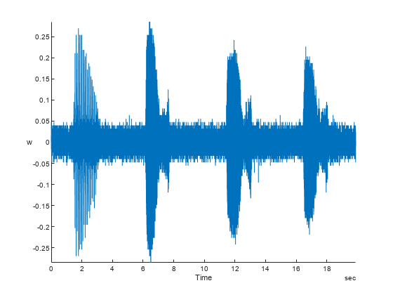
Load a file that contains audio data from a Pacific blue whale, sampled at 4 kHz. The file is from the library of animal vocalizations maintained by the Cornell University Bioacoustics Research Program. The time scale in the data is compressed by a factor of 10 to raise the pitch and make the calls more audible. Convert the signal to a MATLAB® timetable and plot it. Four features stand out from the noise in the signal. The first is known as a trill, and the other three are known as moans.
[w,fs] = audioread('bluewhale.wav');
whale = timetable(w,'SampleRate',fs);
stackedplot(whale);
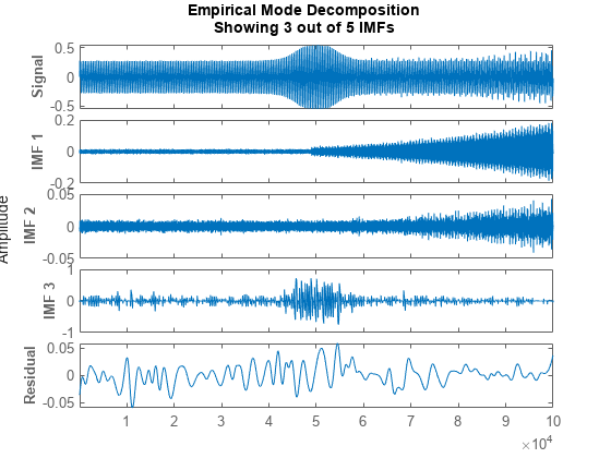
Use emd to visualize the first three intrinsic mode functions (IMFs) and the residual.
emd(whale,'MaxNumIMF',3)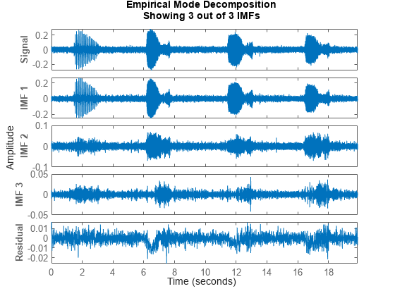
Compute the first three IMFs of the signal. Use the 'Display' name-value pair to output a table showing the number of sifting iterations, the relative tolerance, and the sifting stop criterion for each IMF.
imf = emd(whale,'MaxNumIMF',3,'Display',1);
Current IMF  |  #Sift Iter  |  Relative Tol  |  Stop Criterion Hit
      1      |        1     |      0.13523   |  SiftMaxRelativeTolerance
      2      |        2     |     0.030198   |  SiftMaxRelativeTolerance
      3      |        2     |      0.01908   |  SiftMaxRelativeTolerance
Decomposition stopped because maximum number of intrinsic mode functions was extracted.
Use the computed IMFs to plot the Hilbert spectrum of the signal. Restrict the frequency range from 0 Hz to 1400 Hz.
hht(imf,'FrequencyLimits',[0 1400])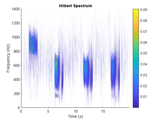
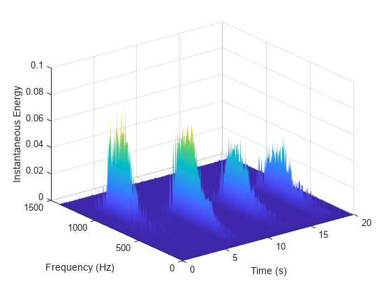
Compute the Hilbert spectrum for the same range of frequencies. Visualize the Hilbert spectra of the trill and moans as a mesh plot.
[hs,f,t] = hht(imf,'FrequencyLimits',[0 1400]);

mesh(seconds(t),f,hs,'EdgeColor','none','FaceColor','interp')
xlabel('Time (s)')
ylabel('Frequency (Hz)')
zlabel('Instantaneous Energy')
Load and visualize a nonstationary continuous signal composed of sinusoidal waves with a distinct change in frequency. The vibration of a jackhammer and the sound of fireworks are examples of nonstationary continuous signals. The signal is sampled at a rate fs.
load("sinusoidalSignalExampleData.mat","X","fs")
t = (0:length(X)-1)/fs;

plot(t,X)
xlabel("Time (s)")
The mixed signal contains sinusoidal waves with different amplitude and frequency values.
To compute the Hilbert spectrum parameters, you need the IMFs of the signal. Perform empirical mode decomposition to compute the intrinsic mode functions and residuals of the signal. Since the signal is not smooth, specify 'pchip' as the interpolation method.
[imf,residual,info] = emd(X,Interpolation="pchip");The table generated in the command window indicates the number of sift iterations, the relative tolerance, and the sift stop criterion for each generated IMF. This information is also contained in info. You can hide the table by specifying 'Display' as 0.
Compute the Hilbert spectrum parameters: Hilbert spectrum hs, frequency vector f, time vector t, instantaneous frequency imfinsf, and instantaneous energy imfinse.
[hs,f,t,imfinsf,imfinse] = hht(imf,fs);
Use the computed Hilbert spectrum parameters for time-frequency analysis and signal diagnostics.
Generate a multicomponent signal consisting of three sinusoids of frequencies 2 Hz, 10 Hz, and 30 Hz. The sinusoids are sampled at 1 kHz for 2 seconds. Embed the signal in white Gaussian noise of variance 0.01².
fs = 1e3;
t = 1:1/fs:2-1/fs;
x = cos(2*pi*2*t) + ...
    2*cos(2*pi*10*t) + ...
    4*cos(2*pi*30*t) + ...
    0.01*randn(1,length(t));
Compute the IMFs of the noisy signal and visualize them in a 3-D plot.
imf = vmd(x);
[p,q] = ndgrid(t,1:size(imf,2));
plot3(p,q,imf)
grid on
xlabel('Time Values')
ylabel('Mode Number')
zlabel('Mode Amplitude')

Use the computed IMFs to plot the Hilbert spectrum of the multicomponent signal. Restrict the frequency range to [0, 40] Hz.
hht(imf,fs,'FrequencyLimits',[0,40])
Simulate a vibration signal from a damaged bearing. Compute the Hilbert spectrum of this signal and look for defects.
A bearing with a pitch diameter of 12 cm has eight rolling elements. Each rolling element has a diameter of 2 cm. The outer race remains stationary as the inner race is driven at 25 cycles per second. An accelerometer samples the bearing vibrations at 10 kHz.
fs = 10000;
f0 = 25;
n = 8;
d = 0.02;
p = 0.12;
The vibration signal from the healthy bearing includes several orders of the driving frequency.
t = 0:1/fs:10-1/fs;
yHealthy = [1 0.5 0.2 0.1 0.05]*sin(2*pi*f0*[1 2 3 4 5]'.*t)/5;
A resonance is excited in the bearing vibration halfway through the measurement process.
yHealthy = (1+1./(1+linspace(-10,10,length(yHealthy)).^4)).*yHealthy;
The resonance introduces a defect in the outer race of the bearing that results in progressive wear. The defect causes a series of impacts that recur at the ball pass frequency outer race (BPFO) of the bearing:
where is the driving rate, is the number of rolling elements, is the diameter of the rolling elements, is the pitch diameter of the bearing, and is the bearing contact angle. Assume a contact angle of 15° and compute the BPFO.
ca = 15;
bpfo = n*f0/2*(1-d/p*cosd(ca));
Use the pulstran function to model the impacts as a periodic train of 5-millisecond sinusoids. Each 3 kHz sinusoid is windowed by a flat top window. Use a power law to introduce progressive wear in the bearing vibration signal.
fImpact = 3000;
tImpact = 0:1/fs:5e-3-1/fs;
wImpact = flattopwin(length(tImpact))'/10;
xImpact = sin(2*pi*fImpact*tImpact).*wImpact;

tx = 0:1/bpfo:t(end);
tx = [tx; 1.3.^tx-2];

nWear = 49e3;
nSamples = 1e5;
yImpact = pulstran(t,tx',xImpact,fs)/5;
yImpact = [zeros(1,nWear) yImpact(1,(nWear+1):nSamples)];
Generate the BPFO vibration signal by adding the impacts to the healthy bearing signal. Plot the signal and select a 0.3-second interval starting at 5.0 seconds.
yBPFO = yImpact + yHealthy;

xLimLeft = 5.0;
xLimRight = 5.3;
yMin = -0.6;
yMax = 0.6;

plot(t,yBPFO)

hold on
[limLeft,limRight] = meshgrid([xLimLeft xLimRight],[yMin yMax]);
plot(limLeft,limRight,"--")
hold off
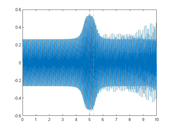
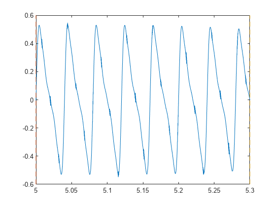
Zoom in on the selected interval to visualize the effect of the impacts.
xlim([xLimLeft xLimRight])
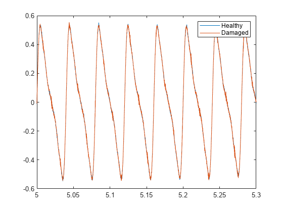
Add white Gaussian noise to the signals. Specify a noise variance of .
rn = 150;
yGood = yHealthy + randn(size(yHealthy))/rn;
yBad = yBPFO + randn(size(yHealthy))/rn;

plot(t,yGood,t,yBad)
xlim([xLimLeft xLimRight])
legend("Healthy","Damaged")
Use emd to perform an empirical mode decomposition of the healthy bearing signal. Compute the first five intrinsic mode functions (IMFs). Use the Display name-value argument to output a table showing the number of sifting iterations, the relative tolerance, and the sifting stop criterion for each IMF.
imfGood = emd(yGood,MaxNumIMF=5,Display=1);
Current IMF  |  #Sift Iter  |  Relative Tol  |  Stop Criterion Hit
      1      |        3     |     0.017132   |  SiftMaxRelativeTolerance
      2      |        3     |      0.12694   |  SiftMaxRelativeTolerance
      3      |        6     |      0.14582   |  SiftMaxRelativeTolerance
      4      |        1     |     0.011082   |  SiftMaxRelativeTolerance
      5      |        2     |      0.03463   |  SiftMaxRelativeTolerance
Decomposition stopped because maximum number of intrinsic mode functions was extracted.
Use emd without output arguments to visualize the first three IMFs and the residual.
emd(yGood,MaxNumIMF=5)
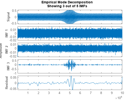
Compute and visualize the IMFs of the defective bearing signal. The first empirical mode reveals the high-frequency impacts. This high-frequency mode increases in energy as the wear progresses.
imfBad = emd(yBad,MaxNumIMF=5,Display=1);
Current IMF  |  #Sift Iter  |  Relative Tol  |  Stop Criterion Hit
      1      |        2     |     0.041274   |  SiftMaxRelativeTolerance
      2      |        3     |      0.16695   |  SiftMaxRelativeTolerance
      3      |        3     |      0.18428   |  SiftMaxRelativeTolerance
      4      |        1     |     0.037177   |  SiftMaxRelativeTolerance
      5      |        2     |     0.095861   |  SiftMaxRelativeTolerance
Decomposition stopped because maximum number of intrinsic mode functions was extracted.
emd(yBad,MaxNumIMF=5)
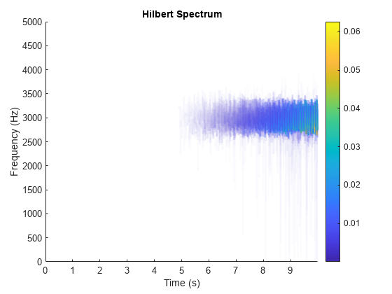
Plot the Hilbert spectrum of the first empirical mode of the defective bearing signal. The first mode captures the effect of high-frequency impacts. The energy of the impacts increases as the bearing wear progresses.
figure
hht(imfBad(:,1),fs)
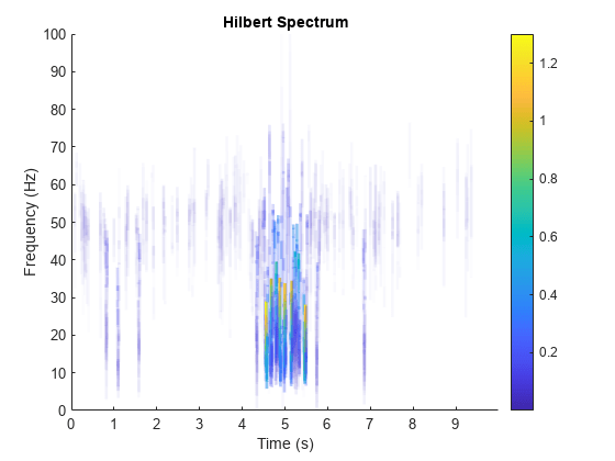
The Hilbert spectrum of the third mode shows the resonance in the vibration signal. Restrict the frequency range from 0 Hz to 100 Hz.
hht(imfBad(:,3),fs,FrequencyLimits=[0 100])
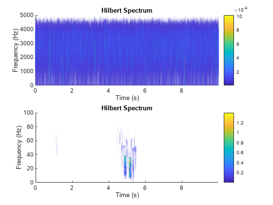
For comparison, plot the Hilbert spectra of the first and third modes of the healthy bearing signal.
subplot(2,1,1)
hht(imfGood(:,1),fs)
subplot(2,1,2)
hht(imfGood(:,3),fs,FrequencyLimits=[0 100])
Input Arguments
Name-Value Arguments
Output Arguments
Algorithms
The Hilbert-Huang transform is useful for performing time-frequency analysis of nonstationary and nonlinear data. The Hilbert-Huang procedure consists of the following steps:
emdorvmddecomposes the data set x into a finite number of intrinsic mode functions.For each intrinsic mode function, xi, the function
hht:Uses
hilbertto compute the analytic signal, , where H{xi} is the Hilbert transform of xi.Expresses zi as , where ai(t) is the instantaneous amplitude and is the instantaneous phase.
Computes the instantaneous energy, , and the instantaneous frequency, . If given a sample rate,
hhtconverts to a frequency in Hz.Outputs the instantaneous energy in
imfinseand the instantaneous frequency inimfinsf.
When called with no output arguments,
hhtplots the energy of the signal as a function of time and frequency, with color proportional to amplitude.
References
[1] Huang, Norden E, and Samuel S P Shen. Hilbert–Huang Transform and Its Applications. 2nd ed. Vol. 16. Interdisciplinary Mathematical Sciences. WORLD SCIENTIFIC, 2014. https://doi.org/10.1142/8804.
[2] Huang, Norden E., Zhaohua Wu, Steven R. Long, Kenneth C. Arnold, Xianyao Chen, and Karin Blank. “ON INSTANTANEOUS FREQUENCY.” Advances in Adaptive Data Analysis 01, no. 02 (April 2009): 177–229. https://doi.org/10.1142/S1793536909000096.