Model and Measure Jitter in SerDes System
This example shows how to use jitter impairments and measurements for serializer/deserializer (SerDes) applications. We will generate a waveform with jitter impairments, measure the total jitter, and estimate the various components that make up that total jitter. We will show various factors that influence accuracy and precision of the total jitter measurement and the various jitter component estimates. Finally, we will discuss the estimation of jitter due to intersymbol interference and additional accuracy and precision concerns unique to the estimation of that jitter component.
Model Jitter
Create an oversampled data waveform with a pseudorandom binary pattern. This example uses a 100 ps unit interval at 16 samples per unit interval. Generate the stimulus waveform using the serdes.Stimulus System Object.
symbolTime = 1e-10; % 1 UI = 100 ps
samplesPerSymbol = 16;
sampleInterval = symbolTime/samplesPerSymbol;
stim = serdes.Stimulus(SymbolTime=symbolTime,SampleInterval=sampleInterval);
Apply Jitter
Use IBIS-AMI jitter parameters to set up TX jitter impairments in the stimulus. Add 5 ps of jitter due to DCD (Duty Cycle Distortion), 10 ps of SJ (Sinusoidal Jitter), and 1 ps RMS of RJ (Random Jitter).
stim.DCD = 5e-12; % 0.05 UI, Half of peak-to-peak DCD
stim.DCDUnit = "Seconds";

stim.Sj = 1e-11; % 0.1 UI, Amplitude of SJ
stim.SjUnit = "Seconds";
stim.SjFrequency = 206e6; % 206 MHz

stim.Rj = 1e-12; % 0.01 UI, Standard deviation of Gaussian random jitter
stim.RjUnit = "Seconds";
Get Waveform
The Stimulus system object generates one sample of data each time it is called. Call the object 16384 times to generate 1024 UI of data, oversampled at 16 samples per symbol.
N = 1024*samplesPerSymbol;
wave = zeros(N,1);
for i = 1:N
    wave(i) = stim();
end
Measure Jitter
Use the function jitter to measure timing error and estimate jitter components. By default, the serdes.Stimulus uses differential signaling and produces a PAM2 waveform, so set SymbolThresholds to 0. Because wave came directly out of the stimulus and did not go through a channel, set ISI to 0 to disable the ISI estimate.
J = jitter(wave, ...
SymbolTime=symbolTime, ...
SampleInterval=sampleInterval, ...
SymbolThresholds=0, ...
ReferenceThresholds=0, ...
ISI=0)
J = struct with fields:
      TJrms: 8.9882e-12
     TJpkpk: 3.5812e-11
      RJrms: 2.8781e-12
      DJrms: 8.8365e-12
     DJpkpk: 3.0033e-11
        SJa: 9.6736e-12
        SJf: 2.0588e+08
        SJp: -1.1486
     DDJrms: 5.3445e-12
    DDJpkpk: 1.0689e-11
     DCDrms: 5.3446e-12
    DCDpkpk: 1.0689e-11
     ISIrms: 0
    ISIpkpk: 0
Compare Impairment and Results
IBIS Tx_DCD is half of the peak-to-peak duty cycle distortion. Therefore, the expected value of the measured DCDpkpk metric is double the DCD impairment. Sj (from the Stimulus) and SJa (from the results) both represent the amplitude of a sinusoid, so their values should be the same. RJrms should also be the similar to the injected amount of Rj as the number of samples goes to infinity.
expected = [2*stim.DCD;stim.Sj;stim.Rj].*1e12; % Convert to ps
actual = [J.DCDpkpk;J.SJa;J.RJrms].*1e12; % Convert to ps
relativeError = (actual - expected)./expected;
disp(table(expected,actual,relativeError,RowNames=["DCD PKPK";"SJ Amplitude";"RJ RMS"]))
                    expected    actual    relativeError
                    ________    ______    _____________

    DCD PKPK           10       10.689       0.068912
    SJ Amplitude       10       9.6736      -0.032641
    RJ RMS              1       2.8781         1.8781
More About Accuracy and Precision
The TJ (Total Jitter) metrics are calculated directly from the timing error sequence. This means that if the edge times from the measured waveform (and reference waveform if applicable) were detected correctly and correctly matched to each other, the TJ measurement is accurate.
The RJ RMS metric is the opposite: the contribution of RJ to the total timing error at each edge is estimated by subtracting the estimates of the other jitter components at that edge from the measured total jitter at that edge. Therefore, any errors in other estimates have an equal and opposite effect on instantaneous RJ and because these effects are uncorrelated with the RJ itself, typically RJ RMS is overestimated to some extent.
DJ and DDJ are combinations of other metrics. For any given edge, DDJ = DCD + ISI and DJ = DDJ + SJ.
SJ is estimated using a discrete Fourier transform (DFT) of the instantaneous jitter values from each edge (the timing error sequence). Accuracy is dependent on how well the frequency of the signal under test aligns with one of the points of the DFT. For amplitude and frequency (SJa and SJf, respectively) the consequences of a mismatch are small relative to the values themselves. For the phase (SJp), however, expect inaccurate results unless the SJ frequency is perfectly centered on a frequency bin. If needed, you can set the number of DFT bins using the NFFT name value pair.
Jitter due to ISI is estimated by recovering a pulse response from the measured data with wave2pulse and then converting that pulse response to an impulse response with pulse2impulse. That impulse response and the symbol pattern of the measured waveform are then used to create a waveform containing only ISI. The timing error at each edge due to ISI is the timing error of the "ISI-only" waveform. Impulse response recovery accuracy is inversely proportional to other jitter sources. To overcome this limitation, supply an impulse response using the ImpulseResponse name value pair. In simulated systems, the impulse response can often be extracted from the channel model. Alternatively, if you have a measured pulse response you can use pulse2impulse. Otherwise, and for measured systems, sParameterFitter allows you to convert s-parameters into impulse responses.
Intersymbol Interference
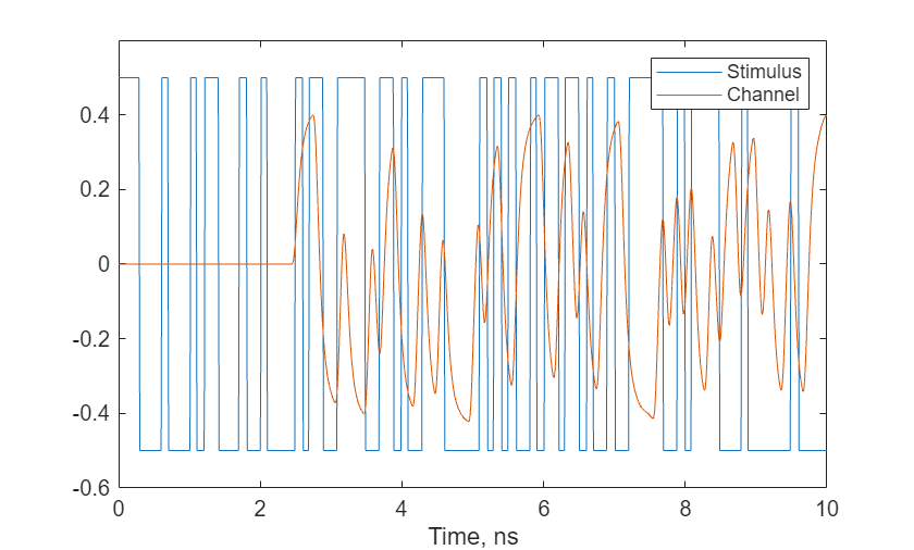
To model ISI, use a serdes.ChannelLoss system object. This system object models an electrical channel based on a loss in dB and a set of electrical characteristics. The dt property value is the time step, so set it to sampleInterval, and the TargetFrequency property value is the frequency of a 1-UI toggle pattern (which is half of the symbol rate). For this example, leave the Loss at its default value of 8 dB.
chan = serdes.ChannelLoss(dt=sampleInterval,TargetFrequency=0.5/symbolTime);
channelImpulse = chan.impulse;
waveISI = chan(wave);
plot((0:length(wave) - 1)*sampleInterval*1e9,[wave,waveISI]);
xlim([0,100*symbolTime*1e9]);
ylim([-0.6,0.6]);
xlabel("Time, ns");
legend("Stimulus","Channel");
Estimate jitter due to ISI in this new waveform. Use the original waveform as the reference to minimize the effects of other jitter types on the recovered impulse response. This process recovers an impulse response from the channel waveform, and works best when the symbol pattern is random or pseudorandom. See wave2pulse and pulse2impulse for details.
[ISIrms,ISIpkpk,~,~,isi,recoveredImpulse] = jitterIntersymbol(waveISI,wave, ...
    SymbolTime=symbolTime, ...
    SampleInterval=sampleInterval, ...
    SymbolThresholds=0, ...
    ReferenceThresholds=0);
fprintf("ISIrms: %g ps\nISIpkpk: %g ps\n",ISIrms*1e12,ISIpkpk*1e12);
ISIrms: 16.6149 ps
ISIpkpk: 111.71 ps
Plot the measured impulse response and the original impairment to compare them.
plot(1:numel(channelImpulse),channelImpulse, ...
1:numel(recoveredImpulse),recoveredImpulse);
xlabel("Sample Index");
legend("Impairment","Measured");
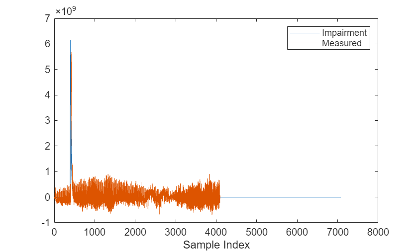
Recovering impulse responses from data with significant DCD, SJ, and/or RJ frequently results in this sort of spurious behavior. Typically, less non-ISI jitter will result in a smaller spur amplitude. Because of this, it is frequently beneficial to measure the channel separately from other jitter metrics.
Now, use the measured impulse response to characterize jitter due to ISI in the context of other jitter metrics. Provide a reference waveform to increase accuracy.
JISIMeasured = jitter(waveISI, ...
    SymbolTime=symbolTime, ...
    SampleInterval=sampleInterval, ...
    SymbolThresholds=0, ...
    ReferenceThresholds=0, ...
    ImpulseResponse=recoveredImpulse);
To compare against the ISI impairment, measure jitter again using the impulse response from the serdes.Stimulus System Object.
JISIImpairment = jitter(waveISI, ...
    SymbolTime=symbolTime, ...
    SampleInterval=sampleInterval, ...
    SymbolThresholds=0, ...
    ReferenceThresholds=0, ...
    ImpulseResponse=channelImpulse);
Display the results in tabular form.
disp(cell2table([struct2cell(J),struct2cell(JISIMeasured),struct2cell(JISIImpairment)], ...
VariableNames=["Tx Out","Channel Out (Measured)", "Channel Out (Impairment)"], ...
RowNames=fieldnames(J)));
                 Tx Out      Channel Out (Measured)    Channel Out (Impairment)
               __________    ______________________    ________________________

    TJrms      8.9882e-12          1.5639e-11                 1.5639e-11
    TJpkpk     3.5812e-11          7.7509e-11                 7.7509e-11
    RJrms      2.8781e-12          1.6512e-11                 1.2114e-11
    DJrms      8.8365e-12          1.7976e-11                 1.4324e-11
    DJpkpk     3.0033e-11          1.1963e-10                 7.0027e-11
    SJa        9.6736e-12          8.7375e-12                 8.7375e-12
    SJf        2.0588e+08          2.1063e+08                 2.1063e+08
    SJp           -1.1486             -2.6008                    -2.6008
    DDJrms     5.3445e-12          1.6916e-11                 1.2754e-11
    DDJpkpk    1.0689e-11          1.0705e-10                 5.8096e-11
    DCDrms     5.3446e-12           6.716e-12                  6.716e-12
    DCDpkpk    1.0689e-11          1.3432e-11                 1.3432e-11
    ISIrms              0          1.5105e-11                 1.1483e-11
    ISIpkpk             0          1.0307e-10                 4.7336e-11
Compare the characterization of ISI using the actual noisy recovered impulse response to the characterization using the same expected impulse response as the Stimulus.
expected = [JISIImpairment.ISIrms;JISIImpairment.ISIpkpk].*1e12; % Convert to ps
actual = [JISIMeasured.ISIrms;JISIMeasured.ISIpkpk].*1e12; % Convert to ps
relativeError = (actual - expected)./expected;
disp(table(expected,actual,relativeError,RowNames=["ISI RMS";"ISI PKPK"]))
                expected    actual    relativeError
                ________    ______    _____________

    ISI RMS      11.483     15.105       0.31544
    ISI PKPK     47.336     103.07        1.1775
Spurious behavior in an impulse response can add up to cause significant shifts in edge timing, and this is captured in the ISI metrics. When using wave2pulse and pulse2impulse to recover an impulse response for jitter characterization, minimize the non-ISI jitter in the waveform to minimize the spurious behavior of the response.