modelDiscriminationPlot
Syntax
Description
modelDiscriminationPlot(___,
specifies options using one or more name-value arguments in addition to the input
arguments in the previous syntax.Name=Value)
h = modelDiscriminationPlot(ax,___,Name=Value)h.
Examples
This example shows how to use fitEADModel to create a Tobit model and then use modelDiscriminationPlot to plot the ROC.
Load EAD Data
Load the EAD data.
load EADData.mat
head(EADData)
UtilizationRate Age Marriage Limit Drawn EAD
_______________ ___ ___________ __________ __________ __________
0.24359 25 not married 44776 10907 44740
0.96946 44 not married 2.1405e+05 2.0751e+05 40678
0 40 married 1.6581e+05 0 1.6567e+05
0.53242 38 not married 1.7375e+05 92506 1593.5
0.2583 30 not married 26258 6782.5 54.175
0.17039 54 married 1.7357e+05 29575 576.69
0.18586 27 not married 19590 3641 998.49
0.85372 42 not married 2.0712e+05 1.7682e+05 1.6454e+05
rng('default');
NumObs = height(EADData);
c = cvpartition(NumObs,'HoldOut',0.4);
TrainingInd = training(c);
TestInd = test(c);
Select Model Type
Select a model type for Tobit or Regression.
ModelType =  "Tobit";
Select Conversion Measure
Select a conversion measure for the EAD response values.
ConversionMeasure =  "LCF";
Create Tobit EAD Model
Use fitEADModel to create a Tobit model using the TrainingInd data.
eadModel = fitEADModel(EADData(TrainingInd,:),ModelType,PredictorVars={'UtilizationRate','Age','Marriage'}, ...
    ConversionMeasure=ConversionMeasure,DrawnVar="Drawn",LimitVar="Limit",ResponseVar="EAD");
disp(eadModel);
Tobit with properties:
CensoringSide: "both"
LeftLimit: 0
RightLimit: 1
ModelID: "Tobit"
Description: ""
UnderlyingModel: [1×1 risk.internal.credit.TobitModel]
PredictorVars: ["UtilizationRate" "Age" "Marriage"]
ResponseVar: "EAD"
LimitVar: "Limit"
DrawnVar: "Drawn"
ConversionMeasure: "lcf"
Display the underlying model. The underlying model's response variable is the transformation of the EAD response data. Use the 'LimitVar' and 'DrawnVar' name-value arguments to modify the transformation.
disp(eadModel.UnderlyingModel);
Tobit regression model:
     EAD_lcf = max(0,min(Y*,1))
     Y* ~ 1 + UtilizationRate + Age + Marriage

Estimated coefficients:
                             Estimate         SE         tStat       pValue
                            __________    __________    _______    __________

    (Intercept)                0.22467      0.031042     7.2377    5.9619e-13
    UtilizationRate             0.4714      0.020681     22.794             0
    Age                     -0.0014209    0.00075695    -1.8772      0.060605
    Marriage_not married     -0.010543      0.015811    -0.6668       0.50496
    (Sigma)                     0.3618     0.0049963     72.414             0

Number of observations: 2627
Number of left-censored observations: 0
Number of uncensored observations: 2626
Number of right-censored observations: 1
Log-likelihood: -1057.9
Predict EAD
EAD prediction operates on the underlying compact statistical model and then transforms the predicted values back to the EAD scale. You can specify the predict function with different options for the 'ModelLevel' name-value argument.
predictedEAD = predict(eadModel,EADData(TestInd,:),ModelLevel="ead");
predictedConversion = predict(eadModel,EADData(TestInd,:),ModelLevel="ConversionMeasure");
Validate EAD Model
For model validation, use modelDiscrimination, modelDiscriminationPlot, modelCalibration, and modelCalibrationPlot.
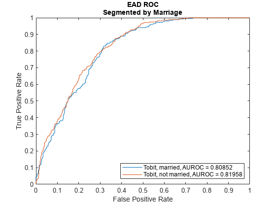
Use modelDiscrimination and then modelDiscriminationPlot to plot the ROC curve.
ModelLevel ="ead"; [DiscMeasure1,DiscData1] = modelDiscrimination(eadModel,EADData(TestInd,:),ModelLevel=ModelLevel); modelDiscriminationPlot(eadModel,EADData(TestInd,:),ModelLevel=ModelLevel,SegmentBy="Marriage");

This example shows how to use fitEADModel to create a Beta model and then use modelDiscriminationPlot to plot the ROC.
Load EAD Data
Load the EAD data.
load EADData.mat
head(EADData)
UtilizationRate Age Marriage Limit Drawn EAD
_______________ ___ ___________ __________ __________ __________
0.24359 25 not married 44776 10907 44740
0.96946 44 not married 2.1405e+05 2.0751e+05 40678
0 40 married 1.6581e+05 0 1.6567e+05
0.53242 38 not married 1.7375e+05 92506 1593.5
0.2583 30 not married 26258 6782.5 54.175
0.17039 54 married 1.7357e+05 29575 576.69
0.18586 27 not married 19590 3641 998.49
0.85372 42 not married 2.0712e+05 1.7682e+05 1.6454e+05
rng('default');
NumObs = height(EADData);
c = cvpartition(NumObs,'HoldOut',0.4);
TrainingInd = training(c);
TestInd = test(c);
Select Model Type
Select a model type for Beta.
ModelType =  "Beta";
Select Conversion Measure
Select a conversion measure for the EAD response values.
ConversionMeasure =  "LCF";
Create Beta EAD Model
Use fitEADModel to create a Beta model using the TrainingInd data.
eadModel = fitEADModel(EADData(TrainingInd,:),ModelType,PredictorVars={'UtilizationRate','Age','Marriage'}, ...
    ConversionMeasure=ConversionMeasure,DrawnVar="Drawn",LimitVar="Limit",ResponseVar="EAD");
disp(eadModel);
Beta with properties:
BoundaryTolerance: 1.0000e-07
ModelID: "Beta"
Description: ""
UnderlyingModel: [1×1 risk.internal.credit.BetaModel]
PredictorVars: ["UtilizationRate" "Age" "Marriage"]
ResponseVar: "EAD"
LimitVar: "Limit"
DrawnVar: "Drawn"
ConversionMeasure: "lcf"
Display the underlying model. The underlying model's response variable is the transformation of the EAD response data. Use the 'LimitVar' and 'DrawnVar' name-value arguments to modify the transformation.
disp(eadModel.UnderlyingModel);
Beta regression model:
     logit(EAD_lcf) ~ 1_mu + UtilizationRate_mu + Age_mu + Marriage_mu
     log(EAD_lcf) ~ 1_phi + UtilizationRate_phi + Age_phi + Marriage_phi

Estimated coefficients:
                                 Estimate        SE         tStat        pValue
                                __________    _________    ________    __________

    (Intercept)_mu                -0.65566      0.11484     -5.7093    1.2615e-08
    UtilizationRate_mu              1.7014     0.078094      21.787             0
    Age_mu                      -0.0055901    0.0027603     -2.0252       0.04295
    Marriage_not married_mu      -0.012576     0.052098     -0.2414       0.80926
    (Intercept)_phi               -0.50131     0.094625     -5.2979    1.2685e-07
    UtilizationRate_phi            0.39731     0.066707       5.956    2.9303e-09
    Age_phi                      -0.001167    0.0023161    -0.50386        0.6144
    Marriage_not married_phi     -0.013275     0.042627    -0.31143        0.7555

Number of observations: 2627
Log-likelihood: -3140.21
Predict EAD
EAD prediction operates on the underlying compact statistical model and then transforms the predicted values back to the EAD scale. You can specify the predict function with different options for the 'ModelLevel' name-value argument.
predictedEAD = predict(eadModel,EADData(TestInd,:),ModelLevel="ead");
predictedConversion = predict(eadModel,EADData(TestInd,:),ModelLevel="ConversionMeasure");
Validate EAD Model
For model validation, use modelDiscrimination, modelDiscriminationPlot, modelCalibration, and modelCalibrationPlot.
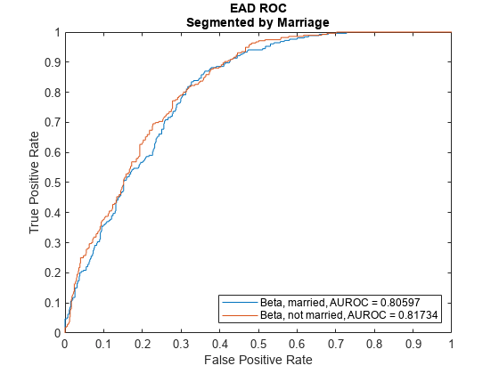
Use modelDiscrimination and then modelDiscriminationPlot to plot the ROC curve.
ModelLevel ="ead"; [DiscMeasure1,DiscData1] = modelDiscrimination(eadModel,EADData(TestInd,:),ModelLevel=ModelLevel); modelDiscriminationPlot(eadModel,EADData(TestInd,:),ModelLevel=ModelLevel,SegmentBy="Marriage");

Input Arguments
Exposure at default model, specified as a previously created Regression,
Tobit, or Beta object using
fitEADModel.
Data Types: object
Data, specified as a
NumRows-by-NumCols table with
predictor and response values. The variable names and data types must be
consistent with the underlying model.
Data Types: table
(Optional) Valid axis object, specified as an ax object
that is created using axes. The plot will be
created in the axes specified by the optional ax argument
instead of in the current axes (gca). The optional argument
ax must precede any of the input argument
combinations.
Data Types: object
Name-Value Arguments
Specify optional pairs of arguments as
Name1=Value1,...,NameN=ValueN, where Name is
the argument name and Value is the corresponding value.
Name-value arguments must appear after other arguments, but the order of the
pairs does not matter.
Example: modelDiscriminationPlot(eadModel,data(TestInd,:),DataID='Testing',DiscretizeBy='median')
Data set identifier, specified as DataID and a
character vector or string. The DataID is included in
the output for reporting purposes.
Data Types: char | string
Discretization method for EAD data at the defined
ModelLevel, specified as
DiscretizeBy and a character vector or string.
'mean'— Discretized response is1if observed EAD is greater than or equal to the mean EAD,0otherwise.'median'— Discretized response is1if observed EAD is greater than or equal to the median EAD,0otherwise.
Data Types: char | string
Name of a column in the data input, not
necessarily a model variable, to be used to segment the data set,
specified as SegmentBy and a character vector or
string. One AUROC is reported for each segment, and the corresponding
ROC data for each segment is returned in the optional output.
Data Types: char | string
Model level, specified as ModelLevel and a
character vector or string.
Note
Regression models support all three model levels,
but a Tobit
or Beta
model supports model levels only for "ead"
and "conversionMeasure".
Data Types: char | string
Identifier for the reference model, specified as
ReferenceID and a character vector or string.
'ReferenceID' is used in the plot for reporting
purposes.
Data Types: char | string
Output Arguments
Figure handle for the line objects, returned as handle object.
More About
The modelDiscriminationPlot function plots the
receiver operator characteristic (ROC) curve.
The modelDiscriminationPlot function also shows the area under
the receiver operator characteristic (AUROC) curve, sometimes called simply the area
under the curve (AUC). This metric is between 0 and 1 and higher values indicate
better discrimination.
A numeric prediction and a binary response are needed to plot the ROC and compute
the AUROC. For EAD models, the predicted EAD is used directly as the prediction.
However, the observed EAD must be discretized into a binary variable. By default,
observed EAD values greater than or equal to the mean observed EAD are assigned a
value of 1, and values below the mean are assigned a value of 0. This discretized
response is interpreted as "high EAD" vs. "low EAD." The ROC curve and the AUROC
curve measure how well the predicted EAD separates the "high EAD" vs. the "low EAD"
observations. You can change the level to compute the model discrimination with the
ModelLevel name-value pair argument and the discretization
criterion with the DiscretizeBy name-value pair
argument.
The ROC curve is a parametric curve that plots the proportion of
High EAD cases with predicted EAD greater than or equal to a parameter t, or true positive rate (TPR)
Low EAD cases with predicted EAD greater than or equal to the same parameter t, or false positive rate (FPR)
The parameter t sweeps through all the observed predicted EAD
values for the given data. If the AUROC value or the ROC curve data are needed
programmatically, use the modelDiscrimination function. For more information about ROC curves,
see ROC Curve and Performance Metrics.
References
[1] Baesens, Bart, Daniel Roesch, and Harald Scheule. Credit Risk Analytics: Measurement Techniques, Applications, and Examples in SAS. Wiley, 2016.
[2] Bellini, Tiziano. IFRS 9 and CECL Credit Risk Modelling and Validation: A Practical Guide with Examples Worked in R and SAS. San Diego, CA: Elsevier, 2019.
[3] Brown, Iain. Developing Credit Risk Models Using SAS Enterprise Miner and SAS/STAT: Theory and Applications. SAS Institute, 2014.
[4] Roesch, Daniel and Harald Scheule. Deep Credit Risk. Independently published, 2020.
Version History
Introduced in R2021bThe eadModel input supports an option for a
Beta model object that you can create using fitEADModel.
MATLAB Command
You clicked a link that corresponds to this MATLAB command:
Run the command by entering it in the MATLAB Command Window. Web browsers do not support MATLAB commands.
Select a Web Site
Choose a web site to get translated content where available and see local events and offers. Based on your location, we recommend that you select: .
You can also select a web site from the following list
How to Get Best Site Performance
Select the China site (in Chinese or English) for best site performance. Other MathWorks country sites are not optimized for visits from your location.
Americas
- América Latina (Español)
- Canada (English)
- United States (English)
Europe
- Belgium (English)
- Denmark (English)
- Deutschland (Deutsch)
- España (Español)
- Finland (English)
- France (Français)
- Ireland (English)
- Italia (Italiano)
- Luxembourg (English)
- Netherlands (English)
- Norway (English)
- Österreich (Deutsch)
- Portugal (English)
- Sweden (English)
- Switzerland
- United Kingdom (English)