modelCalibration
Compute R-square, RMSE, correlation, and sample mean error of predicted and observed EADs
Since R2023a
Syntax
Description
CalMeasure = modelCalibration(eadModel,data)modelCalibration supports comparison against a reference
model and also supports different correlation types. By default,
modelCalibration computes the metrics in the EAD scale. You
can use the ModelLevel name-value argument to compute metrics
using the underlying model's transformed scale.
[
specifies options using one or more name-value arguments in addition to the input
arguments in the previous syntax.CalMeasure,CalData] = modelCalibration(___,Name=Value)
Examples
This example shows how to use fitEADModel to create a Tobit model and then use modelCalibration to compute the R-Square, RMSE, correlation, and sample mean error of predicted and observed EAD.
Load EAD Data
Load the EAD data.
load EADData.mat
head(EADData)
UtilizationRate Age Marriage Limit Drawn EAD
_______________ ___ ___________ __________ __________ __________
0.24359 25 not married 44776 10907 44740
0.96946 44 not married 2.1405e+05 2.0751e+05 40678
0 40 married 1.6581e+05 0 1.6567e+05
0.53242 38 not married 1.7375e+05 92506 1593.5
0.2583 30 not married 26258 6782.5 54.175
0.17039 54 married 1.7357e+05 29575 576.69
0.18586 27 not married 19590 3641 998.49
0.85372 42 not married 2.0712e+05 1.7682e+05 1.6454e+05
rng('default');
NumObs = height(EADData);
c = cvpartition(NumObs,'HoldOut',0.4);
TrainingInd = training(c);
TestInd = test(c);
Select Model Type
Select a model type for Tobit or Regression.
ModelType =  "Tobit";
Select Conversion Measure
Select a conversion measure for the EAD response values.
ConversionMeasure =  "LCF";
Create Tobit EAD Model
Use fitEADModel to create a Tobit model using EADData.
eadModel = fitEADModel(EADData(TrainingInd,:),ModelType,PredictorVars={'UtilizationRate','Age','Marriage'}, ...
    ConversionMeasure=ConversionMeasure,DrawnVar="Drawn",LimitVar="Limit",ResponseVar="EAD");
disp(eadModel);
Tobit with properties:
CensoringSide: "both"
LeftLimit: 0
RightLimit: 1
ModelID: "Tobit"
Description: ""
UnderlyingModel: [1×1 risk.internal.credit.TobitModel]
PredictorVars: ["UtilizationRate" "Age" "Marriage"]
ResponseVar: "EAD"
LimitVar: "Limit"
DrawnVar: "Drawn"
ConversionMeasure: "lcf"
Display the underlying model. The underlying model's response variable is the transformation of the EAD response data. Use the 'LimitVar' and 'DrwanVar' name-value arguments to modify the transformation.
disp(eadModel.UnderlyingModel);
Tobit regression model:
     EAD_lcf = max(0,min(Y*,1))
     Y* ~ 1 + UtilizationRate + Age + Marriage

Estimated coefficients:
                             Estimate         SE         tStat       pValue
                            __________    __________    _______    __________

    (Intercept)                0.22467      0.031504     7.1315    1.2783e-12
    UtilizationRate             0.4714       0.02066     22.817             0
    Age                     -0.0014209    0.00077019    -1.8449      0.065163
    Marriage_not married     -0.010543      0.015835    -0.6658        0.5056
    (Sigma)                     0.3618     0.0049955     72.426             0

Number of observations: 2627
Number of left-censored observations: 0
Number of uncensored observations: 2626
Number of right-censored observations: 1
Log-likelihood: -1057.9
Predict EAD
EAD prediction operates on the underlying compact statistical model and then transforms the predicted values back to the EAD scale. You can specify the predict function with different options for the 'ModelLevel' name-value argument.
predictedEAD = predict(eadModel,EADData(TestInd,:),ModelLevel="ead");
predictedConversion = predict(eadModel,EADData(TestInd,:),ModelLevel="ConversionMeasure");
Validate EAD Model
For model validation, use modelDiscrimination, modelDiscriminationPlot, modelCalibration, and modelCalibrationPlot.
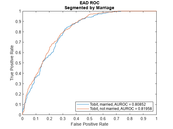
Use modelDiscrimination and then modelDiscriminationPlot to plot the ROC curve.
ModelLevel ="ead"; [DiscMeasure1,DiscData1] = modelDiscrimination(eadModel,EADData(TestInd,:),ModelLevel=ModelLevel); modelDiscriminationPlot(eadModel,EADData(TestInd, :),ModelLevel=ModelLevel,SegmentBy="Marriage");
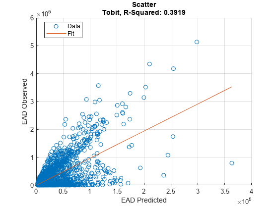
Use modelCalibration, and modelCalibrationPlot to show a scatter plot of the predictions.
YData = "Observed";

[CalMeasure1,CalData1] = modelCalibration(eadModel,EADData(TestInd,:),ModelLevel=ModelLevel)
"Observed";
[CalMeasure1,CalData1] = modelCalibration(eadModel,EADData(TestInd,:),ModelLevel=ModelLevel)CalMeasure1=1×4 table
RSquared RMSE Correlation SampleMeanError
________ _____ ___________ _______________
Tobit 0.3919 42494 0.62602 -1240.7
CalData1=1751×3 table
     Observed     Predicted_Tobit    Residuals_Tobit
    __________    _______________    _______________

         44740           14893              29847
        54.175          8730.2              -8676
        987.39           13244             -12257
        9606.4          7367.5             2238.9
        83.809           27501             -27417
         73538           45726              27812
        96.949          5522.5            -5425.5
        873.21          4426.3            -3553.1
        328.35          5952.4            -5624.1
         55237           28040              27198
         30359           19047              11312
         39211           28368              10843
    2.0885e+05      1.0539e+05         1.0346e+05
        1921.7           19939             -18017
         15230          5427.4             9802.4
         20063          9359.6              10703
      ⋮
modelCalibrationPlot(eadModel,EADData(TestInd,:),ModelLevel=ModelLevel,YData=YData);
This example shows how to use fitEADModel to create a Beta model and then use modelCalibration to compute the R-Square, RMSE, correlation, and sample mean error of predicted and observed EAD.
Load EAD Data
Load the EAD data.
load EADData.mat
head(EADData)
UtilizationRate Age Marriage Limit Drawn EAD
_______________ ___ ___________ __________ __________ __________
0.24359 25 not married 44776 10907 44740
0.96946 44 not married 2.1405e+05 2.0751e+05 40678
0 40 married 1.6581e+05 0 1.6567e+05
0.53242 38 not married 1.7375e+05 92506 1593.5
0.2583 30 not married 26258 6782.5 54.175
0.17039 54 married 1.7357e+05 29575 576.69
0.18586 27 not married 19590 3641 998.49
0.85372 42 not married 2.0712e+05 1.7682e+05 1.6454e+05
rng('default');
NumObs = height(EADData);
c = cvpartition(NumObs,'HoldOut',0.4);
TrainingInd = training(c);
TestInd = test(c);
Select Model Type
Select a model type for Beta.
ModelType =  "Beta";
Select Conversion Measure
Select a conversion measure for the EAD response values.
ConversionMeasure =  "LCF";
Create Beta EAD Model
Use fitEADModel to create a Beta model using the TrainingInd data.
eadModel = fitEADModel(EADData(TrainingInd,:),ModelType,PredictorVars={'UtilizationRate','Age','Marriage'}, ...
    ConversionMeasure=ConversionMeasure,DrawnVar="Drawn",LimitVar="Limit",ResponseVar="EAD");
disp(eadModel);
Beta with properties:
BoundaryTolerance: 1.0000e-07
ModelID: "Beta"
Description: ""
UnderlyingModel: [1×1 risk.internal.credit.BetaModel]
PredictorVars: ["UtilizationRate" "Age" "Marriage"]
ResponseVar: "EAD"
LimitVar: "Limit"
DrawnVar: "Drawn"
ConversionMeasure: "lcf"
Display the underlying model. The underlying model's response variable is the transformation of the EAD response data. Use the 'LimitVar' and 'DrwanVar' name-value arguments to modify the transformation.
disp(eadModel.UnderlyingModel);
Beta regression model:
     logit(EAD_lcf) ~ 1_mu + UtilizationRate_mu + Age_mu + Marriage_mu
     log(EAD_lcf) ~ 1_phi + UtilizationRate_phi + Age_phi + Marriage_phi

Estimated coefficients:
                                Estimate        SE         tStat        pValue
                                _________    _________    ________    __________

    (Intercept)_mu               -0.65566      0.11484     -5.7093    1.2614e-08
    UtilizationRate_mu             1.7014     0.078094      21.787             0
    Age_mu                       -0.00559    0.0027603     -2.0252      0.042952
    Marriage_not married_mu     -0.012576     0.052098     -0.2414       0.80926
    (Intercept)_phi              -0.50132     0.094625     -5.2979    1.2685e-07
    UtilizationRate_phi           0.39731     0.066707       5.956    2.9304e-09
    Age_phi                     -0.001167    0.0023161    -0.50386       0.61441
    Marriage_not married_phi    -0.013275     0.042627    -0.31143        0.7555

Number of observations: 2627
Log-likelihood: -3140.21
Predict EAD
EAD prediction operates on the underlying compact statistical model and then transforms the predicted values back to the EAD scale. You can specify the predict function with different options for the 'ModelLevel' name-value argument.
predictedEAD = predict(eadModel,EADData(TestInd,:),ModelLevel="ead");
predictedConversion = predict(eadModel,EADData(TestInd,:),ModelLevel="ConversionMeasure");
Validate EAD Model
For model validation, use modelDiscrimination, modelDiscriminationPlot, modelCalibration, and modelCalibrationPlot.
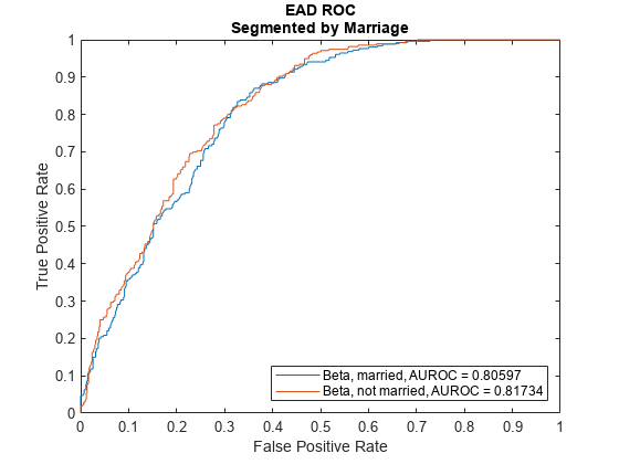
Use modelDiscrimination and then modelDiscriminationPlot to plot the ROC curve.
ModelLevel ="ead"; [DiscMeasure1,DiscData1] = modelDiscrimination(eadModel,EADData(TestInd,:),ModelLevel=ModelLevel); modelDiscriminationPlot(eadModel,EADData(TestInd, :),ModelLevel=ModelLevel,SegmentBy="Marriage");
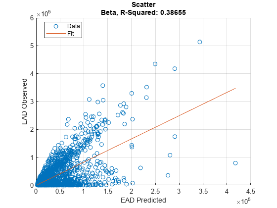
Use modelCalibration, and modelCalibrationPlot to show a scatter plot of the predictions.
YData = "Observed";

[CalMeasure1,CalData1] = modelCalibration(eadModel,EADData(TestInd,:),ModelLevel=ModelLevel)
"Observed";
[CalMeasure1,CalData1] = modelCalibration(eadModel,EADData(TestInd,:),ModelLevel=ModelLevel)CalMeasure1=1×4 table
RSquared RMSE Correlation SampleMeanError
________ _____ ___________ _______________
Beta 0.38655 43817 0.62173 -7393.4
CalData1=1751×3 table
     Observed     Predicted_Beta    Residuals_Beta
    __________    ______________    ______________

         44740           18039           26701
        54.175           10560          -10506
        987.39           15551          -14564
        9606.4          8407.7          1198.8
        83.809           33318          -33234
         73538           52120           21418
        96.949          6598.1         -6501.2
        873.21          5471.1         -4597.9
        328.35            7335         -7006.6
         55237           32580           22658
         30359           21563          8796.4
         39211           33177          6033.6
    2.0885e+05      1.2586e+05           82987
        1921.7           23319          -21397
         15230          6565.9            8664
         20063           11075          8987.5
      ⋮
modelCalibrationPlot(eadModel,EADData(TestInd,:),ModelLevel=ModelLevel,YData=YData);
Input Arguments
Name-Value Arguments
Output Arguments
More About
References
[1] Baesens, Bart, Daniel Roesch, and Harald Scheule. Credit Risk Analytics: Measurement Techniques, Applications, and Examples in SAS. Wiley, 2016.
[2] Bellini, Tiziano. IFRS 9 and CECL Credit Risk Modelling and Validation: A Practical Guide with Examples Worked in R and SAS. San Diego, CA: Elsevier, 2019.
[3] Brown, Iain. Developing Credit Risk Models Using SAS Enterprise Miner and SAS/STAT: Theory and Applications. SAS Institute, 2014.
[4] Roesch, Daniel and Harald Scheule. Deep Credit Risk. Independently published, 2020.
Version History
Introduced in R2023a