Design Matching Network Using Lumped Components from Modelithics Library

This example shows you how to:

• Design a matching network for a reference antenna using ideal components from RF Toolbox™ and real-world components from Modelithics SELECT+ Library™. Ideal components do not take parasitic effects into account. To include these effects in your simulation, you need to build the matching network with real-world components.

• Analyze the ideal and the real-world matching network.

• Compare the performance of the ideal and the real-world matching network with respect to a reference antenna.

The presence of parasitics changes the response of the matching network with real-world lumped components. The non-ideal behavior results from variations in the material properties of the substrate and packing material, solder and pad properties, and orientation.

Video Walkthrough

For a walkthrough of the example, play the video.

Create Inset-Fed Patch Antenna

The first step before designing the matching network for the reference antenna is to design the reference antenna itself. This example uses an inset-fed patch antenna as a reference antenna. Create simple inset-fed patch antenna using the design function from Antenna Toolbox™ implemented on a PCB. Set the antenna dimensions and use an FR4 substrate in this design. And the set the substrate thickness to 0.0014 m.

antennaObject = design(patchMicrostripInsetfed, 2400*1e6);
antennaObject.Length = 0.0265;
antennaObject.Width = 0.0265;
antennaObject.Height = 0.0014;
antennaObject.Substrate.Name = 'FR4';
antennaObject.Substrate.EpsilonR = 4.8;
antennaObject.Substrate.LossTangent = 0.026;
antennaObject.Substrate.Thickness = 0.0014;
antennaObject.FeedOffset = [-0.02835, 0];
antennaObject.StripLineWidth = 0.0016223;
antennaObject.NotchLength = 0.0037853;
antennaObject.NotchWidth = 0.002839;
antennaObject.GroundPlaneLength = 0.0567;
antennaObject.GroundPlaneWidth = 0.0567;

Visualize Inset-Fed Patch Antenna

Use the show function to visualize the structure of this patch antenna.

figure;
show(antennaObject)

Analyze Inset-Fed Patch Antenna

Perform full-wave analysis on the inset-fed patch antenna over 2.3–2.5 GHz and save the S-parameter results to a MAT file. Load the MAT file to view the impedance and reflection coefficient response.

load InsetPatchAntenna.mat
plotFrequency = 2400*1e6;
freqRange = linspace(2.3e9, 2.5e9, 11);

Plot the impedance of the inset-fed patch antenna.

figure;
impedance(antennaObject, freqRange);

Plot the reflection coefficient response of the inset-fed patch antenna.

figure; 
s = sparameters(antennaObject, freqRange);
rfplot(s)

Build Rational Model

Build a rational model for the antenna S-parameter data. This allows you to refine the frequency points in the analysis range and not simulate the antenna again during full-wave analysis.

s_rat = rational(s);
[resp,~] = freqresp(s_rat,freqRange);
hold on
plot(freqRange/1e9,20*log10(abs(resp)))
title('Antenna Reflection Coefficient')
legend('Full-Wave','Rational Model')

Design Matching Network

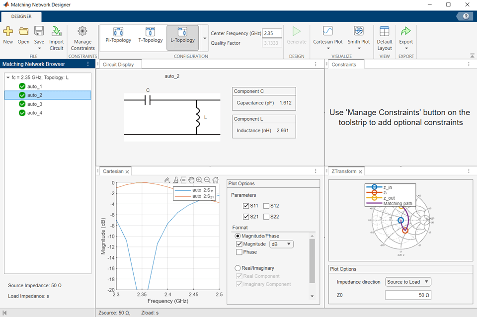
Load the S-parameter data from the workspace to the Matching Network Designer app. Set the matching frequency to 2.35 GHz and the network topology to L-Topology. Once the app generates the networks, select series C, shunt L from the network list and export the network. The app saves the network to MAT file.

To build the matching network, convert the S-parameter data to an nport object and add it to a circuit. Assign ports to the circuit for RF analysis.

ant = nport(s);
load mnapp_LTopo_CserLsh.mat
ckt_lumped = circuit;
add(ckt_lumped,[1 2 0 0],mnckt)
add(ckt_lumped,[2 0],ant)
setports(ckt_lumped,[1 0])

Perform S-Parameters Frequency Sweep

Select 100 points in the analysis frequency range and analyze the matching network response with the antenna S-parameters as the load. Overlay the antenna-only port reflection coefficient over this response. This shifts the antenna response in the lower band to 2.35 GHz.

freqRange = linspace(2.3e9, 2.5e9, 100);
lumped_s = sparameters(ckt_lumped,freqRange);
[resp,freq] = freqresp(s_rat,freqRange);
figure
rfplot(lumped_s,1,1)
hold on
plot(freqRange/1e9,20*log10(abs(resp)))
legend('ANT+Matching N/W','ANT','Location','Best')
title('Reflection Coefficient of Antenna and Matching Network')

Build Matching Network with Non-Ideal Lumped Component Models

Select the non-ideal lumped components from Modelithics Select+ Library. You must have the Modelithics Select+ Library license to run the following code. For more information, see Modelithics SELECT+ Library for MATLAB.

Create RF Component using Modelithics SELECT+ Library

Set up the Modelithics Select+ Library by specifying the full path to the library.

mdlxSetup('C:\mdlx_library\SELECT')

Create the Modelithics library object.

mdlx = mdlxLibrary;

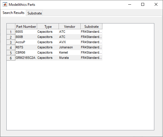
Search the library for a 1.6117 pF capacitor mounted on a 59 mil FR4 substrate. Note that Modelithics components are substrate scalable, and that 59 mil is chosen to match the antenna substrate thickness of 1.4mm.

search(mdlx,'FR4Standard59mil',Type='Capacitors',Value=1.6117e-12)

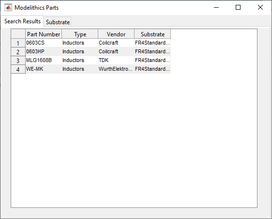
Search the library for a 2.6611 nH inductor mounted on a 59 mil FR4 substrate.

search(mdlx,'FR4Standard59mil',Type='Inductors',Value=2.6611e-9)

Create an array of Modelithics capacitors.

cList = search(mdlx,'FR4Standard59mil',Type='Capacitors',Value=1.6117e-12);

Create an array of Modelithics inductors.

lList = search(mdlx,'FR4Standard59mil',Type='Inductors',Value=2.6611e-9);

Create Matching Network with Modelithics Components

Create a matching network with L-Topology, series C, and shunt L using the first element in the array of Modelithics capacitors and inductors. Most Modelithics lumped components have two ports.

mdlxckt = circuit;
add(mdlxckt,[1 2 0 0],cList(1));
add(mdlxckt,[2 0 0 0],lList(1));
setports(mdlxckt,[1 0],[2 0]);

As with the matching network with ideal lumped components, add the matching network with the Modelithics lumped components and the S-parameters of the inset-fed patch antenna to a circuit. Assign ports to the circuit for RF analysis.

mdlxckt_lumped = circuit;
add(mdlxckt_lumped,[1 2 0 0],mdlxckt)
add(mdlxckt_lumped,[2 0],nport(s))
setports(mdlxckt_lumped,[1 0])

Analyze Matching Network and Antenna

Analyze the matching network response with the antenna S-parameters as the load.

mdlxlumped_s = sparameters(mdlxckt_lumped,freqRange);

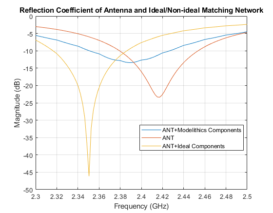
Compare Ideal and Non-Ideal Reflection Coefficients

Overlay the reflection coefficient from the antenna S-parameters with the ones using ideal matching network and the one with real-world components from the Modelithics Select+ Library.

figure
rfplot(mdlxlumped_s,1,1)
hold on
plot(freqRange/1e9,20*log10(abs(resp)))
rfplot(lumped_s,1,1)
legend('ANT+Modelithics Components','ANT','ANT+Ideal Components','Location','Best')
title('Reflection Coefficient of Antenna and Ideal/Non-ideal Matching Network')

Inspect Component Data Sheets

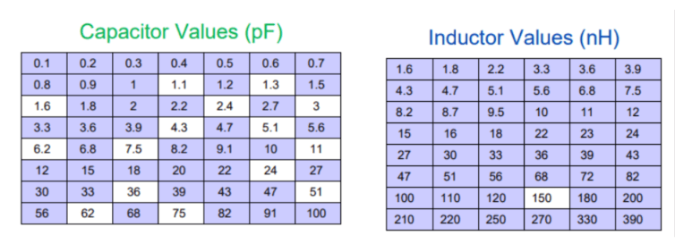
The two L and C components are available only in a limited set of discrete values. Use the datasheet function to inspect their respective data sheets to identify the values that are closer to the nominal values identified before.

datasheet(cList(1));
datasheet(lList(1));

Discrete component values from the data sheets are shown in this figure.

Build Matching Network Using Discrete Component Values

Build a new matching network, and try a few of the discrete values close to the nominal values. The best working values for a matching network operating at 2.35 GHz are 1.3 pF and 1.8 nH. The discrete values are slightly different from the nominal values due to parasitic effects.

c = clone(cList(1));
c.Value = 1.3e-12;
l = clone(lList(1));
l.Value = 1.8e-9;
mdlxcktD = circuit;
add(mdlxcktD,[1 2 0 0],c);
add(mdlxcktD,[2 0 0 0],l);
add(mdlxcktD,[2 0],nport(s))
setports(mdlxcktD,[1 0]);
mdlxlumpeddiscrete_s = sparameters(mdlxcktD,freqRange);

Overlay the reflection coefficient from the ideal matching network, the one with real-world components from the Modelithics Select+ Library using nominal values, and the one with real-world components from the Modelithics Select+ Library using discrete values.

figure
rfplot(mdlxlumpeddiscrete_s,1,1)
hold on
rfplot(mdlxlumped_s,1,1);
rfplot(lumped_s,1,1)
legend('ANT+Modelithics Components Discrete Values', ...
    'ANT+Modelithics Components Nominal Values', ...
    'ANT+Ideal Components','Location','Best')
title('Reflection Coefficient of Antenna and Ideal/Non-ideal Matching Network')

The resulting matching network now works at the target frequency.