Train MBPO Agent to Balance Continuous Cart-Pole System
This example shows how to train a model-based policy optimization (MBPO) agent to balance a continuous action space cart-pole system modeled in MATLAB®. For more information on MBPO agents, see Model-Based Policy Optimization (MBPO) Agent.
MBPO agents use an environment model to generate more experiences while training a base agent. In this example, the base agent is a soft actor-critic (SAC) agent.
The built-in MBPO agent is based on a model-based policy optimization algorithm in [1]. The original MBPO algorithm trains an ensemble of stochastic models. In contrast, this example trains an ensemble of deterministic models. For an example in which an MBPO agent is implemented using a custom training loop, see Model-Based Reinforcement Learning Using Custom Training Loop.
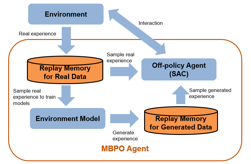
The following figure summarizes the algorithm used in this example. During training the MBPO agent collects real experiences resulting from interactions with the environment. The MBPO agent uses these experiences to train its internal environment model. Then, it uses this model to generate experiences without interacting with the actual environment Finally, the MBPO agent uses the real experiences and generated experiences to train the SAC base agent.
Fix Random Number Stream for Reproducibility
The example code might involve computation of random numbers at several stages. Fixing the random number stream at the beginning of some sections in the example code preserves the random number sequence in the section every time you run it, which increases the likelihood of reproducing the results. For more information, see Results Reproducibility. Fix the random number stream with seed 0 and random number algorithm Mersenne twister. For more information on controlling the seed used for random number generation, see rng.
previousRngState = rng(0,"twister");The output previousRngState is a structure that contains information about the previous state of the stream. You will restore the state at the end of the example.
Cart-Pole MATLAB Environment
For this example, the reinforcement learning environment is a pole attached to an unactuated revolutionary joint on a cart. The cart has an actuated prismatic joint connected to a one-dimensional frictionless track. The training goal in this environment is to balance the pole by applying forces (actions) to the prismatic joint.
For this environment:
The balanced, upright pendulum position is
0radians and the downward hanging pendulum position ispiradians.The pendulum starts upright with an initial angle between –0.05 radians and 0.05 radians.
The force action signal from the agent to the environment is from –10 N to 10 N.
The observations from the environment are the position and velocity of the cart, the pendulum angle (clockwise-politive), and the pendulum angle derivative.
The episode terminates if the pole is more than 12 degrees from vertical or if the cart moves more than 2.4 m from the original position.
A reward of +0.5 is provided for every time-step that the pole remains upright. An additional reward is provided based on the distance between the cart and the origin. A penalty of –50 is applied when the pendulum falls.
For more information on this model, see Use Predefined Control System Environments.
Create a predefined environment object for the cart-pole system.
env = rlPredefinedEnv("CartPole-Continuous");The object has a continuous action space where the agent can apply one force value ranging from –10 N to 10 N.
Obtain the observation and action specifications from the environment object.
obsInfo = getObservationInfo(env);
numObservations = obsInfo.Dimension(1);
actInfo = getActionInfo(env);
Create MBPO Agent
An MBPO agent decides which action to take given observations using a base off-policy agent. The MBPO agent trains both the base agent and an environmental model. The environmental model consists of transition functions, a reward function, and an is-done function. This model is used to create more samples without interacting with an environment. This example uses the following steps to construct an MBPO agent.
Define model-free off-policy agent.
Define transition models.
Define reward model.
Define is-done model.
Create neural network environment.
Create MBPO agent.
1. Define Model-Free Off-Policy Agent
Create a SAC base agent with a default network structure. For more information on SAC agents, see Soft Actor-Critic (SAC) Agent. For an environment with a continuous action space, you can also use a DDPG or TD3 base agent. For discrete environments, you can use a DQN base agent.
agentOpts = rlSACAgentOptions;
agentOpts.MiniBatchSize = 256;
agentOpts.ExperienceBufferLength = 1e6;
agentOpts.NumEpoch = 1;
initOpts = rlAgentInitializationOptions(NumHiddenUnit=128);
baseagent = rlSACAgent(obsInfo,actInfo,initOpts,agentOpts);

baseagent.AgentOptions.ActorOptimizerOptions.LearnRate = 5e-4;
baseagent.AgentOptions.ActorOptimizerOptions.GradientThreshold = 1;
baseagent.AgentOptions.CriticOptimizerOptions(1).LearnRate = 5e-4;
baseagent.AgentOptions.CriticOptimizerOptions(1).GradientThreshold = 1;
baseagent.AgentOptions.CriticOptimizerOptions(2).LearnRate = 5e-4;
baseagent.AgentOptions.CriticOptimizerOptions(2).GradientThreshold = 1;
2. Define Transition Models
To model the environment, an MBPO agent trains one or more transition models. To model an environment effectively, you must consider two kinds of uncertainty: statistical uncertainty and modeling uncertainty. A stochastic transition function can model the statistical uncertainty better than a deterministic transition function. In this example, since the cart-pole environment is deterministic, you use deterministic transition functions.
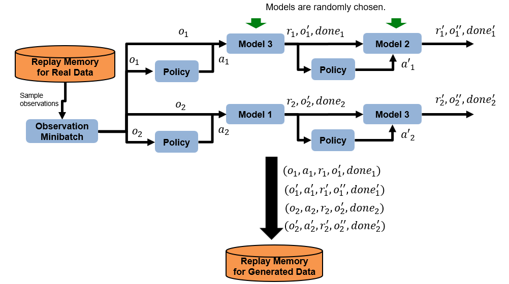
It is challenging to have a perfect model, and a trained model usually has modeling uncertainty. One common approach to overcoming modeling uncertainty is to use multiple transition models. The original MBPO paper uses seven models [1]. For this example, to reduce computational cost, you use three models. The MBPO agent generates experiences using all three transition models. The following figure shows how an ensemble of transition models generates samples without interacting with the environment. In this figure, the models generate two trajectories with horizon = 2.
Create three deterministic transition functions. To do so, create a deep neural network using the createDeterministicTransitionNetwork helper function. Then, use the neural network to create an rlContinuousDeterministicTransitionFunction object. When creating a transition function object, you must specify the action and observation input/output names for the neural network.
net1 = createDeterministicTransitionNetwork(4,1);
transitionFcn1 = rlContinuousDeterministicTransitionFunction(net1, ...
    obsInfo, ...
    actInfo, ...
    ObservationInputNames="state", ...
    ActionInputNames="action", ...
    NextObservationOutputNames="nextObservation");

net2 = createDeterministicTransitionNetwork(4,1);
transitionFcn2 = rlContinuousDeterministicTransitionFunction(net2, ...
    obsInfo, ...
    actInfo, ...
    ObservationInputNames="state", ...
    ActionInputNames="action", ...
    NextObservationOutputNames="nextObservation");

net3 = createDeterministicTransitionNetwork(4,1);
transitionFcn3 = rlContinuousDeterministicTransitionFunction(net3, ...
    obsInfo, ...
    actInfo, ...
    ObservationInputNames="state", ...
    ActionInputNames="action", ...
    NextObservationOutputNames="nextObservation");
3. Define Reward Model
An MBPO agent also contains a reward model for the environment. If you know a ground-truth reward function, you can specify it using a custom function. In this example, the ground-truth reward function is defined in the cartPoleRewardFunction helper function. To use this reward function set useGroundTruthReward to true.
You can also specify a neural-network-based reward function that the MBPO agent can train. In this example, you can use such a reward function by setting useGroundTruthReward to false. The deep neural network for the reward function is defined in the createRewardNetworkActionNextObs helper function. To define an is-done function using the neural network, create an rlContinuousDeterministicRewardFunction object.
useGroundTruthReward = true;
if useGroundTruthReward
    rewardFcn = @cartPoleRewardFunction;
else
    % This neural network uses action and next observation as inputs.
    rewardnet = createRewardNetworkActionNextObs(4,1);
    rewardFcn = rlContinuousDeterministicRewardFunction(rewardnet, ...
        obsInfo, ...
        actInfo, ...
        ActionInputNames="action", ...
        NextObservationInputNames="nextState");
end
4. Define Is-Done Model
An MBPO agent also contains an is-done model for computing the termination signal for the environment. If you know a ground-truth termination signal, you can specify it using a custom function. In this example, the ground-truth termination signal is defined in the cartPoleIsDoneFunction helper function. To use this reward function set useGroundTruthIsDone to true.
You can also specify a neural-network-based is-done function that the MBPO agent can train. In this example, you can use such an is-done function by setting useGroundTruthIsDone to false. The deep neural network for the is-done function is defined in the createIsDoneNetwork helper function. To define an is-done function using the neural network, create an rlIsDoneFunction object.
useGroundTruthIsDone = true;
if useGroundTruthIsDone
    isdoneFcn = @cartPoleIsDoneFunction;
else
    % This neural network uses only next observation as inputs.
    isdoneNet = createIsDoneNetwork(4);
    isdoneFcn = rlIsDoneFunction(isdoneNet, ...
        obsInfo, ...
        actInfo, ...
        NextObservationInputNames="nextState");
end
5. Create Neural Network Environment
Define a neural network environment using the transition, reward, and is-done functions. To do so, create an rlNeuralNetworkEnvironment object.
generativeEnv = rlNeuralNetworkEnvironment( ...
    obsInfo, ...
    actInfo, ...
    [transitionFcn1,transitionFcn2,transitionFcn3], ...
    rewardFcn, ...
    isdoneFcn);

% Reset model environment.
reset(generativeEnv);
6. Create MBPO Agent
Define an MBPO agent using the base off-policy agent and environment model. To do so, first create an MBPO agent options object.
MBPOAgentOpts = rlMBPOAgentOptions;
Specify options for training the environment model. Train the model for 1 epoch at the beginning of each episode and use 15 mini-batches of size 512.
MBPOAgentOpts.NumEpochForTrainingModel = 1;
MBPOAgentOpts.NumMiniBatches = 15;
MBPOAgentOpts.MiniBatchSize = 512;
Specify the ratio of real and generated experience used to train the base SAC agent. For this example, 20% of samples are from the real experience buffer and 80% of samples are from model experience buffer.
MBPOAgentOpts.RealSampleRatio = 0.2;
Specify options for generating samples using the environment model.
Generate 20000 trajectories at the beginning of each epoch.
Use a piecewise roll-out horizon schedule, which increases the horizon length gradually.
Increase the horizon length every 100 epochs.
Use an initial horizon length of 1.
Use a maximum horizon length of 2.
MBPOAgentOpts.ModelRolloutOptions.NumRollout = 20000;
MBPOAgentOpts.ModelRolloutOptions.HorizonUpdateSchedule = "piecewise";
MBPOAgentOpts.ModelRolloutOptions.HorizonUpdateFrequency = 100;
MBPOAgentOpts.ModelRolloutOptions.Horizon = 1;
MBPOAgentOpts.ModelRolloutOptions.HorizonMax = 2;
Specify the size of the model's experience buffer.
MBPOAgentOpts.ModelExperienceBufferLength = 120000;
Specify optimizer options for training the transition models. Use the same optimizer options for all three transition models.
transitionOptimizerOptions1 = rlOptimizerOptions( ...
    LearnRate=5e-4, ...
    GradientThreshold=1.0);
transitionOptimizerOptions2 = rlOptimizerOptions( ...
    LearnRate=5e-4, ...
    GradientThreshold=1.0);
transitionOptimizerOptions3 = rlOptimizerOptions( ...
    LearnRate=5e-4, ...
    GradientThreshold=1.0);
MBPOAgentOpts.TransitionOptimizerOptions = ...
    [transitionOptimizerOptions1, ...
    transitionOptimizerOptions2, ...
    transitionOptimizerOptions3];
Specify optimizer options for training the reward model. If you use a custom ground-truth reward function, the agent ignores these options.
rewardOptimizerOptions = rlOptimizerOptions( ...
    LearnRate=5e-4, ...
    GradientThreshold=1.0);
MBPOAgentOpts.RewardOptimizerOptions = rewardOptimizerOptions;
Specify optimizer options for training the is-done model. If you use a custom ground-truth reward function, the agent ignores these options.
isdoneOptimizerOptions = rlOptimizerOptions( ...
    LearnRate=5e-4, ...
    GradientThreshold=1.0);
MBPOAgentOpts.IsDoneOptimizerOptions = isdoneOptimizerOptions;
Create the MBPO agent, specifying the base agent, environment model, and options.
agent = rlMBPOAgent(baseagent,generativeEnv,MBPOAgentOpts);
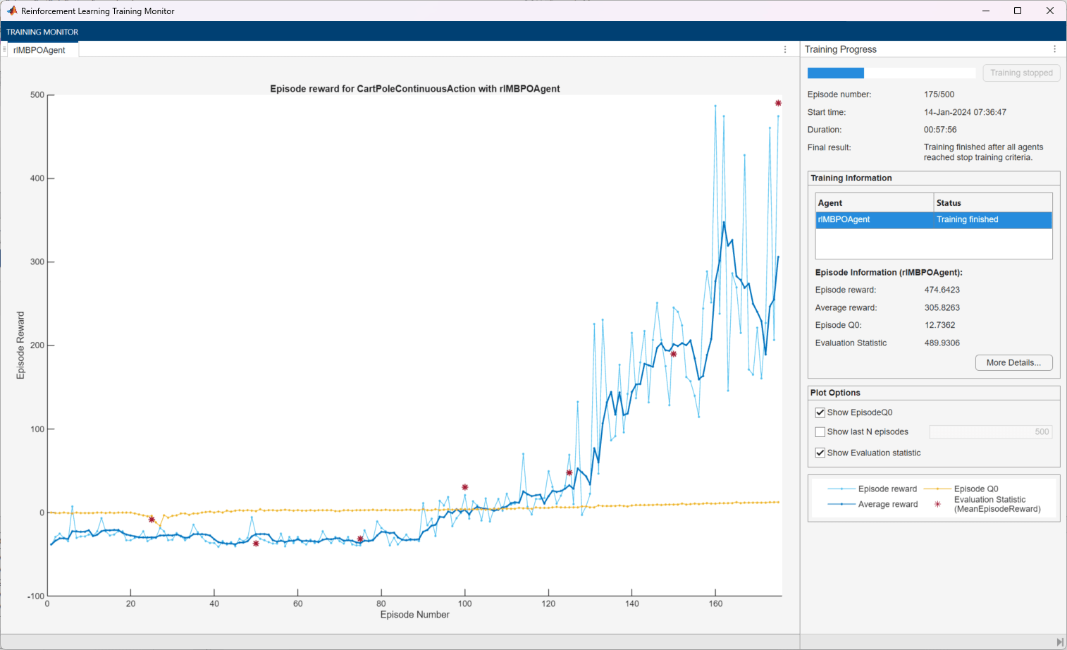
Train Agent
To train the agent, first specify the training options. For this example, use the following options.
Run each training episode for a maximum of 500 episodes, with each episode lasting a maximum of 500 time steps.
Display the training progress in the Reinforcement Learning Training Monitor dialog box (set the
Plotsoption) and disable the command line display (set theVerboseoption tofalse).Save the agent when the average episode reward is greater than or equal to 470.
Stop the training when an evaluation statistic reaches 470. At this point, the agent can balance the pendulum in the upright position.
For more information on training options, see rlTrainingOptions.
trainOpts = rlTrainingOptions( ...
    MaxEpisodes=500, ...
    MaxStepsPerEpisode=500, ...
    Verbose=false, ...
    Plots="training-progress", ...
    StopTrainingCriteria="EvaluationStatistic", ...
    StopTrainingValue=470, ...
    ScoreAveragingWindowLength=5, ...
    SaveAgentCriteria="EpisodeReward", ...
    SaveAgentValue=470);
Create an evaluator object to evaluate the agent using 5 evaluation episodes at every 25 training episodes.
evl = rlEvaluator( ...
    NumEpisodes=5, ...
    EvaluationFrequency=25, ...
    RandomSeeds=101:105);
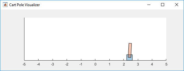
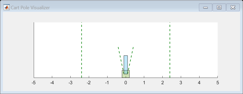
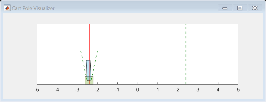
You can visualize the cart-pole system by using the plot function during training or simulation.
plot(env)
Fix the random generator seed for reproducibility.
rng(0);
Train the agent using the train function. Training this agent is a computationally-intensive process that takes several minutes to complete. To save time while running this example, load a pretrained agent by setting doTraining to false. To train the agent yourself, set doTraining to true.
doTraining = false;
if doTraining
    % Train the agent.
    trainingStats = train(agent,env,trainOpts,Evaluator=evl);
else
    % Load the pretrained agent for the example.
    load("MATLABCartpoleMBPO.mat","agent");
end
Simulate MBPO Agent
To validate the performance of the trained agent, simulate it within the cart-pole environment. To make sure you use deterministic actions during the simulation, set the UseExplorationPolicy agent property to agent to be false. For more information on agent simulation, see rlSimulationOptions and sim.
rng(1)

% Make sure exploration is disabled during simulation.
agent.UseExplorationPolicy = false;

simOptions = rlSimulationOptions(MaxSteps=500);
experience = sim(env,agent,simOptions);
totalReward_MBPO = sum(experience.Reward)
totalReward_MBPO = 497.5506
Instead of simulating the MBPO agent, you can simulate the base agent. If you use the same random seed, you get the same result as simulating the MBPO agent.
rng(1)
experience = sim(env,agent.BaseAgent,simOptions);

totalReward_SAC = sum(experience.Reward)
totalReward_SAC =
497.5506
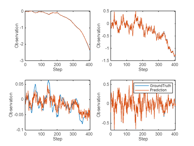
Evaluate Learned Environment Model
To validate the trained environment transition models, you can check whether they are able to correctly predict the next observations. Similarly, you can validate the performance of the reward and is-done functions. To make a prediction based on the environment model, use step.
Collect data for learned model evaluation.
rng(1)

% Enable exploration during sim to create
% diverse data for model evaluation
agent.UseExplorationPolicy = true;

simOptions = rlSimulationOptions(MaxSteps=500);
experience = sim(env,agent,simOptions);
For this example, evaluate the performance of the first transition model.
agent.EnvModel.TransitionModelNum = 1;
For each simulation step, extract the actual next observation.
numSteps = length(experience.Reward.Data);
nextObsPrediction = zeros(4,1,numSteps);
rewardPrediction = zeros(1,numSteps);
isdonePrediction = zeros(1,numSteps);
nextObsGroundTruth = zeros(4,1,numSteps);
rewardGroundTruth = zeros(1,numSteps);
isdoneGroundTruth = zeros(1,numSteps);
for stepCt = 1:numSteps
    % Extract the actual next observation, reward, and is-done value.
    nextObsGroundTruth(:,:,stepCt) = ...
        experience.Observation.CartPoleStates.Data(:,:,stepCt+1);
    rewardGroundTruth(:, stepCt) = experience.Reward.Data(stepCt);
    isdoneGroundTruth(:, stepCt) = experience.IsDone.Data(stepCt);

    % Predict the next observation, reward, and is-done value
    % using the environment model.
    obs = experience.Observation.CartPoleStates.Data(:,:,stepCt);
    agent.EnvModel.Observation = {obs};
    action = experience.Action.CartPoleAction.Data(:,:,stepCt);
    [nextObs,reward,isdone] = step(agent.EnvModel,{action});

    nextObsPrediction(:,:,stepCt) = nextObs{1};
    rewardPrediction(:,stepCt) = reward;
    isdonePrediction(:,stepCt) = isdone;
end
Plot the ground truth and prediction of each dimension of the observations.
figure
for obsDimensionIndex = 1:4
    subplot(2,2,obsDimensionIndex)
    plot(reshape(nextObsGroundTruth(obsDimensionIndex,:,:),1,numSteps))
    hold on
    plot(reshape(nextObsPrediction(obsDimensionIndex,:,:),1,numSteps))
    hold off
    xlabel("Step")
    ylabel("Observation")
    if obsDimensionIndex == 4
        legend("GroundTruth","Prediction","Location","northeast")
    end
end
Restore the random number stream using the information stored in previousRngState.
rng(previousRngState);
References
[1] Janner, Michael, Justin Fu, Marvin Zhang, and Sergey Levine. “When to Trust Your Model: Model-Based Policy Optimization.” In Proceedings of the 33rd International Conference on Neural Information Processing Systems, 12519–30. 1122. Red Hook, NY, USA: Curran Associates Inc., 2019.
See Also
Functions
Objects
rlMBPOAgent|rlNeuralNetworkEnvironment|rlMBPOAgentOptions|rlTrainingOptions|rlSimulationOptions|rlSACAgent