Main Content

plotGratingLobeDiagram

Plot grating lobe diagram of array

Since R2022b

    Description

    example

    plotGratingLobeDiagram(array,freq) plots the grating lobe diagram of an array in the u-v coordinate system. The System object™ array specifies the array. The argument freq specifies the signal frequency. The array, by default, is steered to 0° azimuth and 0° elevation.

    A grating lobe diagram displays the positions of the peaks of the narrowband array pattern. The array pattern depends only upon the geometry of the array and not upon the types of elements which make up the array. Visible and non-visible grating lobes are displayed as open circles. Only grating lobe peaks near the location of the mainlobe are shown. The mainlobe itself is displayed as a filled circle.

    plotGratingLobeDiagram(array,freq,c), in addition, specifies the array steering angle, angle.

    plotGratingLobeDiagram(array,freq,angle,c), in addition, specifies the propagation speed by c.

    plotGratingLobeDiagram(array,freq,angle,c,f0), in addition, specifies an array phase-shifter frequency, f0, that differs from the signal frequency, freq. This argument is useful when the signal no longer satisfies the narrowband assumption and allows you to estimate the size of beam squint.

    hndl = plotGratingLobeDiagram(___) returns the handle hndl to the plot for any of the input syntaxes.

    Examples

    collapse all

    Plot the grating lobe diagram for a 4-element uniform linear array having element spacing less than one-half wavelength. Grating lobes are plotted in u-v coordinates.

    Assume the operating frequency of the array is 3 GHz and the spacing between elements is 0.45 of the wavelength. All elements are isotropic antenna elements. Steer the array in the direction 45 degrees in azimuth and 0 degrees in elevation.

    c = physconst('LightSpeed');
    f = 3e9;
    lambda = c/f;
    sIso = phased.IsotropicAntennaElement;
    sULA = phased.ULA('Element',sIso,'NumElements',4,...
        'ElementSpacing',0.45*lambda);
    plotGratingLobeDiagram(sULA,f,[45;0],c);

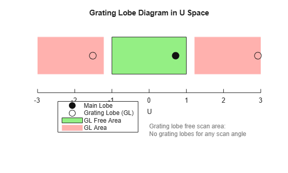
    The main lobe of the array is indicated by a filled black circle. The grating lobes in the visible and nonvisible regions are indicated by empty black circles. The visible region is defined by the direction cosine limits between [-1,1] and is marked by the two vertical black lines. Because the array spacing is less than one-half wavelength, there are no grating lobes in the visible region of space. There are an infinite number of grating lobes in the nonvisible regions, but only those in the range [-3,3] are shown.

    The grating-lobe free region, shown in green, is the range of directions of the main lobe for which there are no grating lobes in the visible region. In this case, it coincides with the visible region.

    The white area of the diagram indicates a region where no grating lobes are possible.

    Input Arguments

    collapse all

    Antenna, microphone, or transducer phased array, specified as a System object.

    Frequencies for computing directivity and patterns, specified as a positive scalar or 1-by-L real-valued row vector. Frequency units are in hertz.

    • For an antenna, microphone, or sonar hydrophone or projector element, FREQ must lie within the range of values specified by the FrequencyRange or FrequencyVector property of the element. Otherwise, the element produces no response and the directivity is returned as –Inf. Most elements use the FrequencyRange property except for phased.CustomAntennaElement and phased.CustomMicrophoneElement, which use the FrequencyVector property.

    • For an array of elements, FREQ must lie within the frequency range of the elements that make up the array. Otherwise, the array produces no response and the directivity is returned as –Inf.

    Example: [1e8 2e6]

    Data Types: double

    Array steering angle, specified as either a 2-by-1 vector or a scalar. If angle is a vector, it takes the form [azimuth;elevation]. The azimuth angle must lie in the range [-180°,180°]. The elevation angle must lie in the range [-90°,90°]. All angle values are specified in degrees. If the argument angle is a scalar, it specifies only the azimuth angle where the corresponding elevation angle is 0°.

    Data Types: double

    Signal propagation speed, specified as a positive scalar. Units are m/s.

    Data Types: double

    Phase-shifter frequency of the array, specified as a scalar. When this argument is omitted, the phase-shifter frequency is assumed to be the signal frequency, freq. Units are Hz

    Data Types: double

    Output Arguments

    collapse all

    Plot handle.

    Algorithms

    collapse all

    Grating Lobes

    Spatial undersampling of a wavefield by an array gives rise to visible grating lobes. If you think of the wavenumber, k, as analogous to angular frequency, then you must sample the signal at spatial intervals smaller than π/kmax (or λmin/2) in order to remove aliasing. The appearance of visible grating lobes is also known as spatial aliasing. The variable kmax is the largest wavenumber value present in the signal.

    The directions of maximum spatial response of a ULA are determined by the peaks of the array’s array pattern (alternatively called the beam pattern or array factor). Peaks other than the mainlobe peak are called grating lobes. For a ULA, the array pattern depends only on the wavenumber component of the wavefield along the array axis (the y-direction for the phased.ULA System object). The wavenumber component is related to the look-direction of an arriving wavefield by ky = –2π sin φ/λ. The angle φ is the broadside angle—the angle that the look-direction makes with a plane perpendicular to the array. The look-direction points away from the array to the wavefield source.

    The array pattern possesses an infinite number of periodically-spaced peaks that are equal in strength to the mainlobe peak. If you steer the array to the φ0 direction, the array pattern for a ULA has its mainlobe peak at the wavenumber value of ky0 = –2π sin φ0. The array pattern has strong grating lobe peaks at kym = ky0 + 2π m/d, for any integer value m. Expressed in terms of direction cosines, the grating lobes occur at um = u0 + mλ/d, where u0 = sin φ0. The direction cosine, u0, is the cosine of the angle that the look-direction makes with the y-axis and is equal to sin φ0 when expressed in terms of the look-direction.

    In order to correspond to a physical look-direction, um must satisfy, –1 ≤ um ≤ 1. You can compute a physical look-direction angle φm from sin φm = um as long as –1 ≤ um ≤ 1. The spacing of grating lobes depends upon λ/d. When λ/d is small enough, multiple grating lobe peaks can correspond to physical look-directions.

    The presence or absence of visible grating lobes for the ULA is summarized in this table.

    Element SpacingGrating Lobes
    λ/d ≥ 2No visible grating lobes for any mainlobe direction.
    1 ≤ λ/d < 2Visible grating lobes can exist for some range of mainlobe directions.
    λ/d < 1Visible grating lobes exist for every mainlobe direction.

    References

    [1] Van Trees, H.L. Optimum Array Processing. New York: Wiley-Interscience, 2002.

    Extended Capabilities

    C/C++ Code Generation
    Generate C and C++ code using MATLAB® Coder™.

    Version History

    Introduced in R2022b

    See Also

    |