plannerMPNET

Create MPNet based bidirectional path planner

Since R2024a

Description

The plannerMPNET object stores a pretrained motion planning networks (MPNet) to use for path planning. MPNet path planner is a bidirectional planner and converges more rapidly towards the optimal solution. The MPNet path planner uses two planning approaches for computing collision-free paths: 1) Bidirectional neural path planning and 2) Classical path planning. The neural path planning method uses a pretrained MPNet to compute the states of a collision-free path. The states computed using neural path planning are called learned states. The classical path planning method uses path planning algorithms such as rapidly-exploring random tree (RRT) method to compute the states of a collision-free path. The states computed using classical path planning are called classical states. By default, the MPNet path planner uses neural path planning to compute optimal path between two states. The planner switches to a classical path planning approach only if the neural path planning method cannot find a path between two states. For information about how the MPNet path planner works, see the Algorithms section.

Creation

Syntax

planner = plannerMPNET(stateValidator,mpnet)

planner = plannerMPNET(___,Name=Value)

Description

planner = plannerMPNET(stateValidator,mpnet) creates a bidirectional MPNet path planner using a state validator and pretrained MPNet.

• The stateValidator argument sets the StateValidator property of the MPNet path planner.

• The mpnet argument sets the MotionPlanningNetwork property of the MPNet path planner.

planner = plannerMPNET(___,Name=Value) specifies the MaxLearnedStates and ClassicalPlannerFcn properties of the MPNet path planner using name-value arguments.

Note

To run this function, you will require the Deep Learning Toolbox™.

Properties

StateValidator — State validator for planner

validatorVehicleCostmap | validatorOccupancyMap | object of a subclass from nav.StateValidator class

This property is read-only.

State validator for the MPNet path planner, specified as a validatorVehicleCostmap object, validatorOccupancyMap object, or an object of the subclass from nav.StateValidator class.

MotionPlanningNetwork — Pretrained MPNet

mpnetSE2 object

This property is read-only.

Pretrained MPNet for neural path planning, specified as an mpnetSE2 object. The MPNet path planner converges more rapidly towards the optimal solution if the pretrained network is trained on optimal paths. For more information about MPNet, see Get Started with Motion Planning Networks.

MaxLearnedStates — Maximum number of learned states

50 (default) | positive scalar integer

Maximum number of learned states to be generated by the MPNet path planner, specified as a positive scalar integer. If this value is set to zero, the MPNet path planner defaults to using a classical path planning method, as specified by the ClassicalPlannerFcn property.

Data Types: single | double | int8 | int16 | int32 | int64 | uint8 | uint16 | uint32 | uint64

ClassicalPlannerFcn — Classical planner for planning

plannerRRTStar (default) | function handle

Classical planner for planning, specified as a function handle to call any of these path planners: plannerRRT, plannerBiRRT, or plannerRRTStar object. The path planner resorts to a classical planner in the following cases:

1. Maximum number of learned states is set to 0.

2. Maximum number of learned states is insufficient to compute a path between the start and goal points.

3. One or more consecutive states in the global path, returned by the MPNet, collide with an obstacle. For more information about how planner recomputes the path in the presence of collisions, see the Algorithms section.

By default, the planner uses the RRT* path planning algorithm if pretrained MPNet fails to generate a path. This property is visible only when you specify ClassicalPlannerFcn as an input.

Data Types: function_handle

Object Functions

plan	Find obstacle-free path between two states
copy	Create deep copy of MPNet path planner object

Examples

Plan Path Between Two States Using MPNet Path Planner

Load Pretrained MPNet

Load a data file containing a pretrained MPNet into the MATLAB® workspace. The MPNet has been trained on various 2-D maze maps with widths and heights of 10 meters and resolutions of 2.5 cells per meter. Each maze map contains a passage width of 5 grid cells and wall thickness of 1 grid cell.

data = load("mazeMapTrainedMPNET.mat")

data = struct with fields:
      encodingSize: [9 9]
       lossWeights: [100 100 0]
        mazeParams: {[5]  [1]  'MapSize'  [10 10]  'MapResolution'  [2.5000]}
       stateBounds: [3x2 double]
    trainedNetwork: [1x1 dlnetwork]

Set the seed value to generate repeatable results.

rng(10,"twister")

Create Maze Map for Motion Planning

Create a random maze map for motion planning. The grid size ($\mathrm{MapSize}\times \mathrm{MapResolution}$) must be same as that of the maps used for training the MPNet.

map = mapMaze(5,1,MapSize=[10 10],MapResolution=2.5);

Create State Validator

Create a state validator object to use for motion planning.

stateSpace = stateSpaceSE2(data.stateBounds);
stateValidator = validatorOccupancyMap(stateSpace,Map=map);
stateValidator.ValidationDistance = 0.1;

Select Start and Goal States

Generate multiple random start and goal states by using the sampleStartGoal function.

[startStates,goalStates] = sampleStartGoal(stateValidator,100);

Compute distance between the generated start and goal states.

stateDistance= distance(stateSpace,startStates,goalStates);

Select two states that are farthest from each other as the start and goal for motion planning.

[dist,index] = max(stateDistance);
start = startStates(index,:);
goal = goalStates(index,:);

Visualize the input map.

figure
show(map)
hold on
plot(start(1),start(2),plannerLineSpec.start{:})
plot(goal(1),goal(2),plannerLineSpec.goal{:})
legend(Location="bestoutside")
hold off

Compute Path Using MPNet Path Planner

Configure the mpnetSE2 object to use the pretrained MPNet for path planning. Set the EncodingSize property values of the mpnetSE2 object to that of the value used for training the network.

mpnet = mpnetSE2(Network=data.trainedNetwork,StateBounds=data.stateBounds,EncodingSize=data.encodingSize);

Create MPNet path planner using the state validator and the pretrained MPNet.

planner = plannerMPNET(stateValidator,mpnet);

Plan a path between the select start and goal states using the MPNet path planner.

[pathObj,solutionInfo] = plan(planner,start,goal);

Display Planned Path

Display the navPath object returned by the MPNet path planner. The number of states in the planned path and the associated state vectors are specified by the NumStates and States properties of the navPath object, respectively.

disp(pathObj)

  navPath with properties:

      StateSpace: [1x1 stateSpaceSE2]
          States: [5x3 double]
       NumStates: 5
    MaxNumStates: Inf

Set the line and marker properties to display the start and goal states by using the plannerLineSpec.start and plannerLineSpec.goal functions, respectively.

sstate = plannerLineSpec.start(DisplayName="Start state",MarkerSize=6);
gstate = plannerLineSpec.goal(DisplayName="Goal state",MarkerSize=6);

Set the line properties to display the computed path by using the plannerLineSpec.path function.

ppath = plannerLineSpec.path(LineWidth=1,Marker="o",MarkerSize=8,MarkerFaceColor="white",DisplayName="Planned path");

Plot the planned path.

figure
show(map)
hold on
plot(pathObj.States(:,1),pathObj.States(:,2),ppath{:})
plot(start(1),start(2),sstate{:})
plot(goal(1),goal(2),gstate{:})
legend(Location="bestoutside")
hold off

Display Additional Data

Display the solutionInfo structure returned by the MPNet path planner. This structure stores the learned states, classical states, and beacon states computed by the MPNet path planner. If any of these three types of states are not computed by the MPNet path planner, the corresponding field value is set to empty.

disp(solutionInfo)

        IsPathFound: 1
      LearnedStates: [50x3 double]
       BeaconStates: [2x3 double]
    ClassicalStates: [9x3 double]

Set the line and marker properties to display the learned states, classical states, and beacon states by using the plannerLineSpec.state.

lstate = plannerLineSpec.state(DisplayName="Learned states",MarkerSize=3);
cstate = plannerLineSpec.state(DisplayName="Classical states",MarkerSize=3,MarkerFaceColor="green",MarkerEdgeColor="green");
bstate = plannerLineSpec.state(MarkerEdgeColor="magenta",MarkerSize=7,DisplayName="Beacon states",Marker="^");

Plot the learned states, classical states, and beacon states along with the computed path. From the figure, you can infer that the neural path planning approach was unable to compute a collision-free path where beacon states are present. Hence, the MPNet path planner resorted to the classical RRT* path planning approach. The final states of the planned path constitutes states returned by neural path planning and classical path planning approaches.

figure
show(map)
hold on
plot(pathObj.States(:,1),pathObj.States(:,2),ppath{:})
plot(solutionInfo.LearnedStates(:,1),solutionInfo.LearnedStates(:,2),lstate{:})
plot(solutionInfo.ClassicalStates(:,1),solutionInfo.ClassicalStates(:,2),cstate{:})
plot(solutionInfo.BeaconStates(:,1),solutionInfo.BeaconStates(:,2),bstate{:})
plot(start(1),start(2),sstate{:})
plot(goal(1),goal(2),gstate{:})
legend(Location="bestoutside")
hold off

Modify Classical Planning Approach for MPNet Path Planner

Load Pretrained MPNet

Load a data file containing a pretrained MPNet into the MATLAB® workspace. The MPNet has been trained on various 2-D maze maps with widths and heights of 10 meters and resolutions of 2.5 cells per meter. Each maze map contains a passage width of 5 grid cells and wall thickness of 1 grid cell.

data = load("mazeMapTrainedMPNET.mat")

data = struct with fields:
      encodingSize: [9 9]
       lossWeights: [100 100 0]
        mazeParams: {[5]  [1]  'MapSize'  [10 10]  'MapResolution'  [2.5000]}
       stateBounds: [3x2 double]
    trainedNetwork: [1x1 dlnetwork]

Set the seed value to generate repeatable results.

rng(70,"twister")

Create Maze Map for Motion Planning

Create a random maze map for motion planning. The grid size ($\mathrm{MapSize}\times \mathrm{MapResolution}$) must be same as that of the maps used for training the MPNet.

map = mapMaze(5,1,MapSize=[12 12],MapResolution=2.0833);

Create State Validator

Create a state validator object to use for motion planning.

stateSpace = stateSpaceSE2(data.stateBounds);
stateValidator = validatorOccupancyMap(stateSpace,Map=map);
stateValidator.ValidationDistance = 0.1;

Select Start and Goal States

Select a start and goal state by using the sampleStartGoal function.

[startStates,goalStates] = sampleStartGoal(stateValidator,500);

Compute distance between the generated start and goal states.

stateDistance= distance(stateSpace,startStates,goalStates);

Select two states that are farthest from each other as the start and goal for motion planning.

[dist,index] = max(stateDistance);
start = startStates(index,:);
goal = goalStates(index,:);

Create MPNet Path Planner

Configure the mpnetSE2 object to use the pretrained MPNet for path planning. Set the EncodingSize property values of the mpnetSE2 object to that of the value used for training the network.

mpnet = mpnetSE2(Network=data.trainedNetwork,StateBounds=data.stateBounds,EncodingSize=data.encodingSize);

Create MPNet path planner using the state validator and the pretrained MPNet. Plan a path between the select start and goal states using the MPNet path planner.

planner{1} = plannerMPNET(stateValidator,mpnet);
[pathObj1,solutionInfo1] = plan(planner{1},start,goal)

pathObj1 = 
  navPath with properties:

      StateSpace: [1x1 stateSpaceSE2]
          States: [6x3 double]
       NumStates: 6
    MaxNumStates: Inf

solutionInfo1 = struct with fields:
        IsPathFound: 1
      LearnedStates: [50x3 double]
       BeaconStates: [2x3 double]
    ClassicalStates: [20x3 double]

Create Copy of MPNet Path Planner

Create a copy of the first instance of the MPNet path planner.

planner{2} = copy(planner{1});

Modify Classical Path Planning Approach

Specify bi-directional RRT (Bi-RRT) planner as the classical path planning approach for MPNet path planner. Set the maximum connection distance value to 1.

classicalPlanner = plannerBiRRT(stateSpace,stateValidator,MaxConnectionDistance=1);
planner{2}.ClassicalPlannerFcn = @classicalPlanner.plan;

Plan a path between the select start and goal states using the modified MPNet path planner.

[pathObj2,solutionInfo2] = plan(planner{2},start,goal)

pathObj2 = 
  navPath with properties:

      StateSpace: [1x1 stateSpaceSE2]
          States: [5x3 double]
       NumStates: 5
    MaxNumStates: Inf

solutionInfo2 = struct with fields:
        IsPathFound: 1
      LearnedStates: [50x3 double]
       BeaconStates: [2x3 double]
    ClassicalStates: [7x3 double]

Visualize Results

Set the line and marker properties to display the start and goal states by using the plannerLineSpec.start and plannerLineSpec.goal functions, respectively.

sstate = plannerLineSpec.start(DisplayName="Start state",MarkerSize=6);
gstate = plannerLineSpec.goal(DisplayName="Goal state",MarkerSize=6);

Set the line and marker properties to display the computed by using the plannerLineSpec.path function.

ppath1 = plannerLineSpec.path(LineWidth=1,Marker="o",MarkerSize=8,MarkerFaceColor="white",DisplayName="Path computed using RRT* for classical path planning");
ppath2 = plannerLineSpec.path(LineWidth=1,Marker="o",MarkerSize=8,MarkerFaceColor="red",DisplayName="Path computed using Bi-RRT for classical path planning");

Plot the computed paths. You can infer that the MPNet path planner offers better results when you use Bi-RRT path planner for classical path planning.

figure
show(map)
hold on
plot(pathObj1.States(:,1),pathObj1.States(:,2),ppath1{:})
plot(pathObj2.States(:,1),pathObj2.States(:,2),ppath2{:})
plot(start(1),start(2),sstate{:})
plot(goal(1),goal(2),gstate{:})
legend(Location="southoutside")
hold off

Plan Path in Dubins State Space Using MPNet Path Planner

Load a data file containing a pretrained MPNet into MATLAB® workspace. The MPNet has been trained on a single map for a Dubins vehicle. You can use this pretrained MPNet to find compute paths between any start state and goal state on the map used for training.

inputData = load("officeMapTrainedMPNET.mat")

inputData = struct with fields:
      encodingSize: 0
       lossWeights: [100 100 10]
        officeArea: [1x1 occupancyMap]
    trainedNetwork: [1x1 dlnetwork]

Read the map used for training the network.

map = inputData.officeArea;

Specify the limits of the state space variables corresponding to the input map.

x = map.XWorldLimits;
y = map.YWorldLimits;
theta = [-pi pi];
stateBounds = [x; y; theta];

Create a Dubins state space and set the minimum turning radius to 0.2.

stateSpace = stateSpaceDubins(stateBounds);
stateSpace.MinTurningRadius = 0.2;

Create a state validator object to use for motion planning. Set the validation distance to 0.1 m.

stateValidator = validatorOccupancyMap(stateSpace,Map=map);
stateValidator.ValidationDistance = 0.1;

Set the seed value to generate repeatable results.

rng(100,"twister");

Generate multiple random start and goal states by using the sampleStartGoal function.

[startStates,goalStates] = sampleStartGoal(stateValidator,500);

Compute distance between the generated start and goal states.

stateDistance= distance(stateSpace,startStates,goalStates);

Select two states that are farthest from each other as the start and goal for motion planning.

[dist,index] = max(stateDistance);
start = startStates(index,:);
goal = goalStates(index,:);

Configure the mpnetSE2 object to use the pretrained MPNet for predicting state samples between a start pose and goal pose. Set the EncodingSize value to 0.

mpnet = mpnetSE2(Network=inputData.trainedNetwork,StateBounds=stateBounds,EncodingSize=0);

Create MPNet path planner using the state validator and the pretrained MPNet.

planner = plannerMPNET(stateValidator,mpnet);

Plan a path between the select start and goal states using the MPNet path planner.

[pathObj,solutionInfo]  = plan(planner,start,goal)

pathObj = 
  navPath with properties:

      StateSpace: [1x1 stateSpaceDubins]
          States: [5x3 double]
       NumStates: 5
    MaxNumStates: Inf

solutionInfo = struct with fields:
        IsPathFound: 1
      LearnedStates: [23x3 double]
       BeaconStates: [4x3 double]
    ClassicalStates: [0x3 double]

Set the line and marker properties to display the start and goal states by using the plannerLineSpec.start and plannerLineSpec.goal functions, respectively.

sstate = plannerLineSpec.start(DisplayName="Start state",MarkerSize=6);
gstate = plannerLineSpec.goal(DisplayName="Goal state",MarkerSize=6);

Set the line properties to display the computed path by using the plannerLineSpec.path function.

ppath = plannerLineSpec.path(LineWidth=1,Marker="o",MarkerSize=8,MarkerFaceColor="white",DisplayName="Planned path");

Display the input map, and plot the start and goal poses.

figure
show(map)
hold on
plot(pathObj.States(:,1),pathObj.States(:,2),ppath{:})
plot(start(1),start(2),sstate{:})
plot(goal(1),goal(2),gstate{:})
legend(Location="bestoutside")
hold off

Display the solutionInfo structure returned by the MPNet path planner. This structure stores the learned states, classical states, and beacon states computed by the MPNet path planner. If any of these three types of states are not computed by the MPNet path planner, the corresponding field value is set to empty.

disp(solutionInfo)

        IsPathFound: 1
      LearnedStates: [23x3 double]
       BeaconStates: [4x3 double]
    ClassicalStates: [0x3 double]

Set the line and marker properties to display the learned states and beacon states by using the plannerLineSpec.state.

lstate = plannerLineSpec.state(DisplayName="Learned states",MarkerSize=3);
bstate = plannerLineSpec.state(MarkerEdgeColor="magenta",MarkerSize=7,DisplayName="Beacon states",Marker="^");

Plot the learned states and beacon states along with the computed path. From the figure, you can infer that the neural path planning approach successfully computed a collision-free path in two places where beacon states are present. Hence, the MPNet path planner did not resort to the classical RRT* path planning approach. The final states of the planned path are the ones returned by the neural path planning approach.

figure
show(map)
hold on
plot(pathObj.States(:,1),pathObj.States(:,2),ppath{:})
plot(solutionInfo.LearnedStates(:,1),solutionInfo.LearnedStates(:,2),lstate{:})
plot(solutionInfo.BeaconStates(:,1),solutionInfo.BeaconStates(:,2),bstate{:})
plot(start(1),start(2),sstate{:})
plot(goal(1),goal(2),gstate{:})
legend(Location="bestoutside")
hold off

Train MPNet on Custom Data for Motion Planning

This example shows how to train a MPNet on a custom dataset and then use the trained network for computing paths between two states in an unknown map environment.

Load and Visualize Training Data set

Load the data set from a .mat file. The data set contains 400,000 different paths for 200 maze map environments. The data set has been generated for a pre-defined parameters of mazeMap function. The first column of the data set contains the maps and the second column contains the optimal paths for randomly sampled start, goal states from the corresponding maps. The size of data set is 75MB.

% Download and extract the maze map dataset
if ~exist("mazeMapDataset.mat","file")
    datasetURL = "https://ssd.mathworks.com/supportfiles/nav/data/mazeMapDataset.zip";
    websave("mazeMapDataset.zip", datasetURL);
    unzip("mazeMapDataset.zip")
end

% Load the maze map dataset
load("mazeMapDataset.mat","dataset","stateSpace")
head(dataset)

             Map                  Path     
    ______________________    _____________

    1×1 binaryOccupancyMap    {14×3 single}
    1×1 binaryOccupancyMap    { 8×3 single}
    1×1 binaryOccupancyMap    {24×3 single}
    1×1 binaryOccupancyMap    {23×3 single}
    1×1 binaryOccupancyMap    {17×3 single}
    1×1 binaryOccupancyMap    {15×3 single}
    1×1 binaryOccupancyMap    { 7×3 single}
    1×1 binaryOccupancyMap    {10×3 single}

The data set was generated using the examplerHelperGenerateDataForMazeMaps helper function. The examplerHelperGenerateDataForMazeMaps helper function uses the mapMaze function to generate random maze maps of size 10-by-10 and resolution 2.5 m. The width and wall thickness of the maps was set to 5m and 1 m, respectively.

passageWidth = 5;
wallThickness = 1;
map = mapMaze(passageWidth,wallThickness,MapSize=[10 10],MapResolution=2.5)

Then, the start states and goal states are randomly generated for each map. The optimal path between the start and goal states are computed using plannerRRTStar path planner. The ContinueAfterGoalReached and MaxIterations parameters are set to true and 5000, respectively, to generate the optimal paths.

planner = plannerRRTStar(stateSpace,stateValidator); % Uses default uniform state sampling
planner.ContinueAfterGoalReached = true; % Optimize after goal is reached
planner.MaxIterations = 5000; % Maximum iterations to run the planner

Visualize a few random samples from the training data set. Each sample contains a map and the optimal path generated for a given start and goal state.

figure
for i=1:4
    subplot(2,2,i)
    ind = randi(height(dataset)); % Select a random sample
    map = dataset(ind,:).Map; % Get map from Map column of the table
    pathStates = dataset(ind,:).Path{1}; % Get path from Path column of the table
    start = pathStates(1,:);
    goal = pathStates(end,:);

    % Plot the data
    show(map);
    hold on
    plot(pathStates(:,1),pathStates(:,2),plannerLineSpec.path{:})
    plot(start(1),start(2),plannerLineSpec.start{:})
    plot(goal(1),goal(2),plannerLineSpec.goal{:})
end
legend(Location="bestoutside")

You can modify the helper function to generate new maps and train the MPNet from scratch. The dataset generation may take a few days depending upon CPU configuration and the number of maps you want to generate for training. To accelerate dataset generation, you can use Parallel Computing Toolbox™.

Create Motion Planning Networks

Create Motion Planning Networks (MPNet) object for SE(2) state space using mpnetSE2. The mpnetSE2 object loads a preconfigured MPNet that you can use for training. Alternatively, you can use the mpnetLayers function to create a MPNet with different number of inputs and hidden layers to train on the data set.

mpnet = mpnetSE2;

Set the StateBounds, LossWeights, and EncodingSize properties of the mpnetSE2 object. Set the StateBounds using the StateBounds property of the stateSpace object.

mpnet.StateBounds = stateSpace.StateBounds;

Specify the weights for each state space variables using the LossWeights property of the mpnetSE2 object. You must specify the weights for each state space variable $\mathit{x}$, $\mathit{y}$, and $\theta$ of SE(2) state space. For a SE(2) state space, we do not consider the robot kinematics such as the turning radius. Hence, you can assign zero weight value for the $\theta$ variable.

mpnet.LossWeights = [100 100 0];

Specify the value for EncodingSize property of the mpnetSE2 object as [9 9]. Before training the network, the mpnetSE2 object encodes the input map environments to a compact representation of size 9-by-9.

mpnet.EncodingSize = [9 9];

Prepare Data for Training

Split the dataset into train and test sets in the ratio 0.8:0.2. The training set is used to train the Network weights by minimizing the training loss, validation set is used to check the validation loss during the training.

split = 0.8;
trainData = dataset(1:split*end,:);
validationData = dataset(split*end+1:end,:);

Prepare the data for training by converting the raw data containing the maps and paths into a format required to train the MPNet.

dsTrain = mpnetPrepareData(trainData,mpnet);
dsValidation = mpnetPrepareData(validationData,mpnet);

Visualize prepared dataset. The first column of sample contains the encoded map data, encoded current state and goal states. The second column contains the encoded next state. The encoded state is computed as $[x,y,\cos (\theta ),\sin (\theta \left)\right]$ and normalized to the range of [0, 1].

preparedDataSample = read(dsValidation);
preparedDataSample(1,:)

ans=1×2 cell array
    {[0.2607 0.4112 0.6846 0.9647 0.9138 0.5757 0.4883 1.3733e-04 0.0549 0.1646 0 0.1646 0.1646 0.1646 0.1646 0.1646 0.0549 0.1646 0.8244 0.0870 0.9383 0.8244 0.8244 0.8244 0.8244 0.1646 0.1646 0.8244 0.0870 0.9020 0.0094 0.0870 0.0870 0.0870 3.9316e-16 0.1646 0.8244 0.0870 0.9020 0.0094 0.9020 0.9043 0.9383 0.1646 0.1646 0.8244 0.0870 0.9020 0.0094 0.9020 0.0870 0.8244 0.1646 0.1646 1 0.9043 0.9020 0.0094 0.9020 0.0870 0.8244 0.1646 0.1646 0.8313 0.0870 0.0870 0.0094 0.9020 0.0870 0.8244 0.1646 0.1646 0.9333 0.8244 0.8244 0.8244 0.9383 0.0870 0.8244 0.1646 0.0549 0.1646 0.1646 0.1646 0.1646 0.1646 2.6928e-16 0.1646 0.0549]}    {[0.2720 0.4130 0.6786 0.9670]}

Train Deep Learning Network

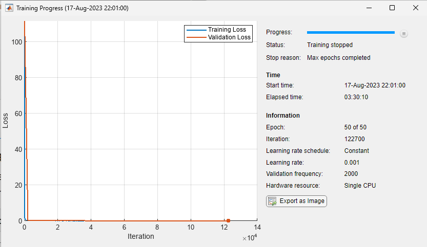
Use the trainnet function to train the MPNet. Training this network might take a long time depending on the hardware you use. Set the doTraining value to true to train the network.

doTraining = false;

Specify trainingOptions (Deep Learning Toolbox) for training the deep learning network:

• Set "adam" optimizer.

• Set the MiniBatchSize for training to 2048.

• Shuffle the dsTrain at every epoch.

• Set the MaxEpochs to 50.

• Set the ValidationData to dsValidation and ValidationFrequency to 2000.

You can consider the training to be successful once the training loss and validation loss converge close to zero.

if doTraining
    options = trainingOptions("adam",...
        MiniBatchSize=2048,...
        MaxEpochs=50,...
        Shuffle="every-epoch",...
        ValidationData=dsValidation,...
        ValidationFrequency=2000,...
        Plots="training-progress");

    % Train network
    [net,info] = trainnet(dsTrain,mpnet.Network,@mpnet.loss,options);

    % Update Network property of mpnet object with net
    mpnet.Network = net;
end

You can save the trained network and the details of input map environment to a .mat file and use it to perform motion planning. In the rest of example, you will use a pretrained MPNet to directly perform motion planning on an unknown map environment.

Load a .mat file containing the pretrained network. The network has been trained on various, randomly generated maze maps stored in the mazeMapDataset.mat file. The .mat file contains the trained network and details of the maze maps used for training the network.

if ~doTraining
    data = load("mazeMapTrainedMPNET.mat")
    mpnet.Network = data.trainedNetwork;
end

data = struct with fields:
      encodingSize: [9 9]
       lossWeights: [100 100 0]
        mazeParams: {[5]  [1]  'MapSize'  [10 10]  'MapResolution'  [2.5000]}
       stateBounds: [3×2 double]
    trainedNetwork: [1×1 dlnetwork]

Perform Motion Planning Using Trained MPNet

Create a random maze map for testing the trained MPNet for path panning. The grid size (MapSize×MapResolution) of the test map must be same the as that of the maps used for training the MPNet.

Click the Run button to generate a new map.

 
mazeParams = data.mazeParams;
map = mapMaze(mazeParams{:});
figure
show(map)

Create a state validator object.

stateValidator = validatorOccupancyMap(stateSpace,Map=map);
stateValidator.ValidationDistance = 0.1;

Create a MPNet path planner using the state validator and the MPNet object as inputs.

planner = plannerMPNET(stateValidator,mpnet);

Generate multiple random start and goal states by using the sampleStartGoal function.

[startStates,goalStates] = sampleStartGoal(stateValidator,500);

Compute distance between the generated start and goal states.

stateDistance=distance(stateSpace,startStates,goalStates);

Select two states that are farthest from each other as the start and goal for motion planning.

[dist,index] = max(stateDistance);
start = startStates(index,:);
goal = goalStates(index,:);

Plan path between the start and goal states using the trained MPNet.

[pathObj,solutionInfo] = plan(planner,start,goal)

pathObj = 
  navPath with properties:

      StateSpace: [1×1 stateSpaceSE2]
          States: [6×3 double]
       NumStates: 6
    MaxNumStates: Inf

solutionInfo = struct with fields:
        IsPathFound: 1
      LearnedStates: [32×3 double]
       BeaconStates: [2×3 double]
    ClassicalStates: [0×3 double]

Set the line and marker properties to display the start and goal states by using the plannerLineSpec.start and plannerLineSpec.goal functions, respectively.

sstate = plannerLineSpec.start(DisplayName="Start state",MarkerSize=6);
gstate = plannerLineSpec.goal(DisplayName="Goal state",MarkerSize=6);

Set the line properties to display the computed path by using the plannerLineSpec.path function.

ppath = plannerLineSpec.path(LineWidth=1,Marker="o",MarkerSize=8,MarkerFaceColor="white",DisplayName="Planned path");

Plot the planned path.

figure
show(map)
hold on
plot(pathObj.States(:,1),pathObj.States(:,2),ppath{:})
plot(start(1),start(2),sstate{:})
plot(goal(1),goal(2),gstate{:})
legend(Location="bestoutside")
hold off

Algorithms

The plan function of the plannerMPNET object implements the MPNet path planning algorithm presented in [1]. This section gives a brief overview of the algorithm.

• The MPNet path planner computes a coarse path consisting of learned states that lie along the global path between start and goal states. If the path connecting any learned states is not collision-free, the MPNet path planner performs replanning only for that segment in the coarse path.

• Two consecutive learned states that are in the free space and cannot be connected without colliding with an obstacle are termed beacon states. The MPNet path planner selects these beacon states as new start and goal points and attempts to find a collision-free path to connect them. This step is referred to as replanning. The path planner makes a limited number of attempts to find this path. If it is not able to find the path within a specified number of attempts, it switches to using a classical path planner. The MPNet path planner determines the maximum number of attempts it can make before switching to a classical planner by using the MaxNumLearnedStates property.

• At every planning and replanning step, the planner applies the lazy states contraction (LSC) approach to remove redundant states computed by the planner. This results in reduced computational complexity and helps the planner find the shortest collision-free path between the actual start and goal states.

References

[1] Qureshi, Ahmed Hussain, Yinglong Miao, Anthony Simeonov, and Michael C. Yip. “Motion Planning Networks: Bridging the Gap Between Learning-Based and Classical Motion Planners.” IEEE Transactions on Robotics 37, no. 1 (February 2021): 48–66. https://doi.org/10.1109/TRO.2020.3006716.

Extended Capabilities

C/C++ Code Generation

Generate C and C++ code using MATLAB® Coder™.

• To use a custom path planner in code generation workflow, the ClassicalPlannerFcn property must be set to a custom function handle before calling the plan function and it cannot be changed after initialization.

Version History

Introduced in R2024a