Compute Functional Connectivity from Brain fMRI
This example shows how to compute resting state networks from resting-state fMRI (R-fMRI) using seed-based cross-correlation with seeds labeled in the Medical Image Labeler app.
Functional magnetic resonance imaging (fMRI) of the brain is a dynamic MRI that measures the level of blood and oxygen supplied to different regions of the brain over a period of time. Because fMRI is a 4-D spatiotemporal signal acquired over a period of time, it can be used to assess the functional health of the brain. Regions of the brain that usually function together show functional connectivity even in the resting state. You can measure functional connectivity in the form of normalized cross-correlations of fMRI timeseries with the timeseries of a seed region. You can select the seed region from a corresponding anatomical MRI scan, as it is easier to visualize compared to an fMRI scan. In this example, you perform these steps to compute the resting-state functional connectivity in the visual cortex of the brain from fMRI.
Label the seed region in an anatomical MRI using the Medical Image Labeler app.
Compute the resting-state functional connectivity in the brain with the seed region by using the resting-state fMRI data.
Visualize the resting-state functional connectivity map overlaid on the anatomical MRI.
Download Data Set
This example uses the resting-state fMRI and anatomical MRI data of one subject from the Human Connectome Project (HCP) Young Adult data set [1][2]. Perform these steps to download the preprocessed data of one subject.
Create an account on the BALSA platform by providing the required details.
Log in to the BALSA platform.
Switch to the ConnectomeDB tab in the BALSA library.
Select the HCP-Young Adult 2025 data set.
Install the IBM Aspera Connect client as prompted.
Accept the Data Use Terms.
Select the Single Subject subject group.
Queue and download the Resting State fMRI 3T Preprocessed Recommended imaging package to the current working directory.
The data set is a ZIP file named 100307_Rest3TRecommended.zip, and has a size of approximately 10GB. Unzip the data set.
unzip("100307_Rest3TRecommended.zip")Load Resting-state fMRI Data
Import the resting-state fMRI data as a medicalVolume object. Observe that the fMRI data has a spatial size of 91-by-109-by-91 and 1200 timepoints.
fMRI = medicalVolume("100307/MNINonLinear/Results/rfMRI_REST1_LR/rfMRI_REST1_LR_hp2000_clean_rclean_tclean.nii.gz");
[h,w,d,T] = size(fMRI.Voxels)
h = 91
w =
109
d =
91
T =
1200
Extract the voxels of the fMRI data and reshape them into a matrix, named fMRIVoxelsMatrix, such that every column of the matrix represents one timepoint of the fMRI data.
fMRIVoxels = fMRI.Voxels;
fMRIVoxelsMatrix = reshape(fMRI.Voxels,[],T);
Label Seed Region
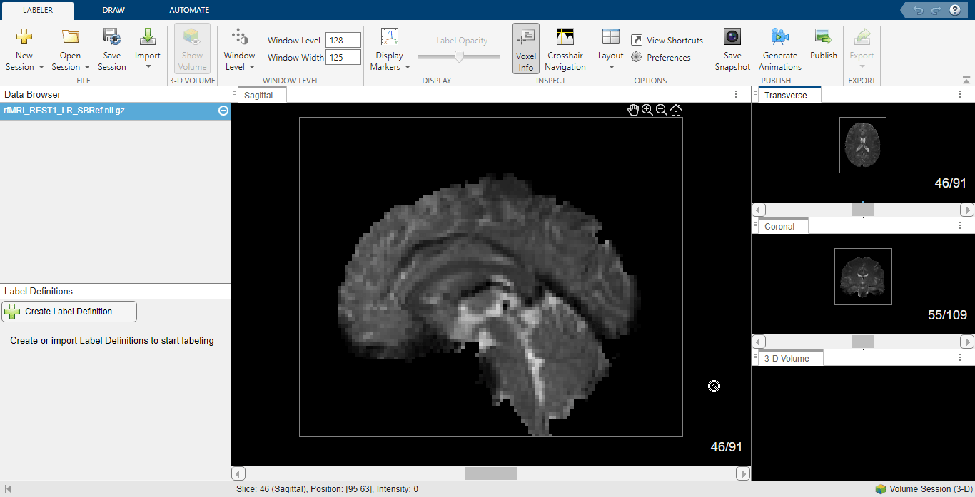
To label the seed region, open the Medical Image Labeler app.
medicalImageLabeler
On the Labeler tab of the app toolstrip, click New Session and select New Volume session (3-D). In the dialog box that opens, specify the current working directory as the session folder, and click Create Session. On the Labeler Tab, select Import and, under Data, select From File. In the dialog box that opens, select the zipped anatomical MRI NIfTI file rfMRI_REST1_LR_SBRef.nii located in the same location as the fMRI NIfTI file, and click Open. On the Labeler tab, select the Voxel Info. Then click Layout and select your desired view. This example computes the resting-state functional connectivity map for the visual cortex, and thus uses the sagittal view to label the seed region in the visual cortex of the brain.
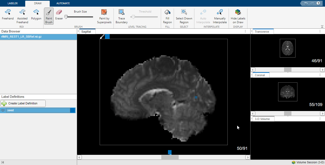
In the Label Definitions pane, select Create Label Definition and name it seed. On the Draw tab of the app toolstrip, select Paint Brush and use the Brush Size parameter to choose the smallest brush size. Label the seed region in the visual cortex. On the Labeler tab of the app toolstrip, select Save Session and close the app.
Compute Functional Connectivity Map
Read the label data from the medical image labeling session using the niftiread function. The label data is a mask for the selected seed region. Reshape the mask into a single column and convert it to logical values.
seedMask = niftiread("MedicalLabelingSession/LabelData/rfMRI_REST1_LR_SBRef.nii");
seedMask = reshape(seedMask,[],1);
seedMask = logical(seedMask);
Use the reshaped mask as a logical index to get the timeseries of the seed voxels from fMRIVoxelsMatrix. Compute the mean seed timeseries from the timeseries of the selected seed voxels.
seed = fMRIVoxelsMatrix(seedMask,:);
seed = mean(seed);
Compute the resting-state functional connectivity map from the voxels of the fMRI data and the seed timeseries using the computeRestingStateFunctionalConnectivity supporting function, defined at the end of this example. The function returns a 3-D volume that is a mask of the regions functionally connected with the seed region.
funcConnMap = computeRestingStateFunctionalConnectivity(fMRIVoxels,seed);
Visualize Functional Connectivity Map on Anatomical MRI
Read the anatomical MRI using the niftiread function, and rescale it for better visualization.
anat = niftiread("100307/MNINonLinear/Results/rfMRI_REST1_LR/rfMRI_REST1_LR_SBRef.nii.gz");
anat = anat/max(anat(:));
Extract sagittal, transverse, and coronal slices to visualize from the anatomical MRI and from the functional connectivity map. Overlay each slice of the functional connectivity map onto the corresponding slice of the anatomical MRI, and reorder the dimensions for better visualization. Visualize the functional connectivity map overlaid on the anatomical MRI.
sagittal_slice = 49;
anat_slice = squeeze(anat(sagittal_slice,:,:));
funcConnMap_slice = squeeze(funcConnMap(sagittal_slice,:,:));
I = labeloverlay(anat_slice,funcConnMap_slice,Colormap="hsv");
I = permute(I,[2 1 3]);
I = I(end:-1:1,end:-1:1,:);
figure
imshow(I)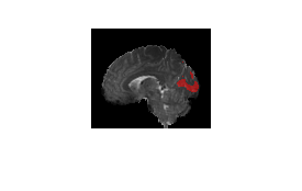
transverse_slice = 41;
anat_slice = squeeze(anat(:,:,transverse_slice));
funcConnMap_slice = squeeze(funcConnMap(:,:,transverse_slice));
J = labeloverlay(anat_slice,funcConnMap_slice,Colormap="hsv");
J = permute(J,[2 1 3]);
J = J(end:-1:1,:,:);
figure
imshow(J)
coronal_slice = 27;
anat_slice = squeeze(anat(:,coronal_slice,:));
funcConnMap_slice = squeeze(funcConnMap(:,coronal_slice,:));
K = labeloverlay(anat_slice,funcConnMap_slice,Colormap="hsv");
K = permute(K,[2 1 3]);
K = K(end:-1:1,:,:);
figure
imshow(K)
Supporting Function
The computeRestingStateFunctionalConnectivity supporting function computes the resting-state functional connectivity map from the voxels of the fMRI data and the seed timeseries. The function computes the strength of the normalized cross-correlation of the seed timeseries with the timeseries at each voxel. The function smooths and rescales the correlation map to reduce the effect of noise on the correlation map. Finally, the function thresholds the correlation map. If the strength of the correlation at a particular voxel is more than 0.5, the function considers the voxel to be functionally connected to the seed region.
function funcConnMap = computeRestingStateFunctionalConnectivity(V,seed)
    [h,w,d,T] = size(V);
    funcConnMap=zeros(h,w,d);
    mask = mean(V,4)~=0;
    for p = 1:1:d
        for n = 1:1:w
            for m = 1:1:h
                if mask(m,n,p) > 0
                    c = corrcoef(seed,V(m,n,p,:));
                    funcConnMap(m,n,p) = abs(c(1,2));
                end
            end
        end
    end
    funcConnMap = smooth3(funcConnMap,"gaussian",5,5);
    funcConnMap = funcConnMap/max(funcConnMap(:));
    funcConnMap = funcConnMap>0.5;
end
References
[1] Data were provided [in part] by the Human Connectome Project, WU-Minn Consortium (Principal Investigators: David Van Essen and Kamil Ugurbil; 1U54MH091657) funded by the 16 NIH Institutes and Centers that support the NIH Blueprint for Neuroscience Research; and by the McDonnell Center for Systems Neuroscience at Washington University.
[2] Van Essen, D.C., K. Ugurbil, E. Auerbach, D. Barch, T.E.J. Behrens, R. Bucholz, A. Chang, et al. “The Human Connectome Project: A Data Acquisition Perspective.” NeuroImage 62, no. 4 (October 2012): 2222–31. https://doi.org/10.1016/j.neuroimage.2012.02.018.