waterfall

Waterfall plot

• 

Syntax

waterfall(X,Y,Z)

waterfall(X,Y,Z,C)

waterfall(Z)

waterfall(Z,C)

waterfall(___,Name=Value)

waterfall(ax,___)

p = waterfall(___)

Description

waterfall(X,Y,Z) creates a waterfall plot, which is a mesh plot with a partial curtain along the y dimension. This results in a "waterfall" effect. The function plots the values in matrix Z as heights above a grid in the xy-plane defined by X and Y. The edge colors vary according to the heights specified by Z.

waterfall(X,Y,Z,C) additionally specifies the color of the edges.

waterfall(Z) creates a waterfall plot, and uses the column and row indices of the elements in Z as the x- and y-coordinates.

waterfall(Z,C) additionally specifies the color of the edges.

waterfall(___,Name=Value) sets properties of the waterfall plot using one or more name-value arguments. For example, you can specify the color and thickness of the plot edges. For a list of properties, see Patch Properties. (since R2024b)

waterfall(ax,___) plots into the axes specified by ax instead of the current axes. Specify the axes as the first input argument. This argument can be used with any of the previous input syntaxes.

p = waterfall(___) returns the patch object. Use p to modify the waterfall plot after it is created. For a list of properties, see Patch Properties.

Examples

Create Waterfall Plot

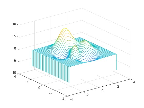
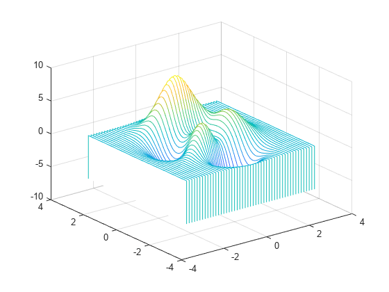
Create three matrices of the same size. Then plot them as a waterfall plot. The mesh plot uses Z for both height and color.

[X,Y] = meshgrid(-3:.125:3);
Z = peaks(X,Y);
waterfall(X,Y,Z)

Specify Colormap Colors

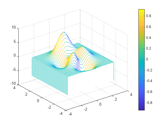
Specify the colors for a waterfall plot by including a fourth matrix input, C. The waterfall plot uses Z for height and C for color. Add a color bar to the graph to show how the data values in C correspond to the colors in the colormap.

[X,Y] = meshgrid(-3:.125:3);
Z = peaks(X,Y);
C = gradient(Z);
waterfall(X,Y,Z,C)
colorbar

Modify Plot Appearance

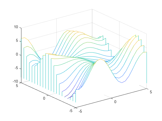
Create a waterfall plot. To allow further modifications, assign the patch object to the variable p.

[X,Y] = meshgrid(-5:.5:5);
Z = Y.*sin(X) - X.*cos(Y);
p = waterfall(X,Y,Z)

p = 
  Patch with properties:

    FaceColor: [1 1 1]
    FaceAlpha: 1
    EdgeColor: 'flat'
    LineStyle: '-'
        Faces: [21x26 double]
     Vertices: [546x3 double]

  Use GET to show all properties

Use p to access and modify properties of the waterfall plot after it is created. For example, change the color of the plot edges by setting the EdgeColor property.

p.EdgeColor = 'b';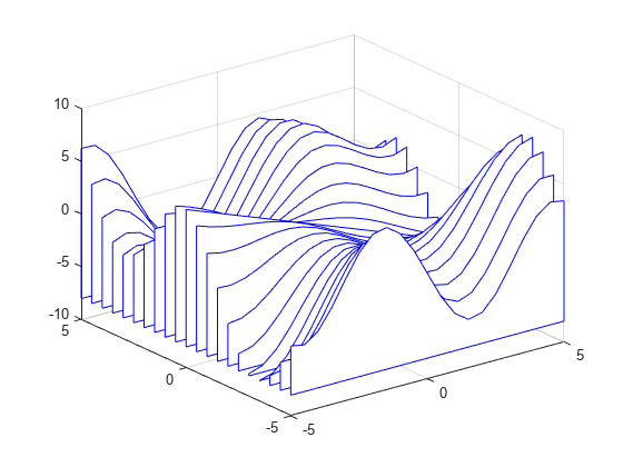

Change Curtain Location

Display a partial curtain along the x-dimension (instead of the y-dimension) by transposing the input arguments.

[X,Y] = meshgrid(-3:.125:3);
Z = peaks(X,Y);
waterfall(X',Y',Z')

Input Arguments

X — x-coordinates

matrix | vector

x-coordinates, specified as a matrix the same size as Z, or as a vector with length n when Z is an m-by-n matrix. If you do not specify values for X and Y, waterfall uses the vectors (1:n) and (1:m).

The XData property of the patch object stores the x-coordinates.

Example: X = 1:10

Example: X = [1 2 3; 1 2 3; 1 2 3]

Example: [X,Y] = meshgrid(-5:0.5:5)

Data Types: single | double | int8 | int16 | int32 | int64 | uint8 | uint16 | uint32 | uint64 | categorical

Y — y-coordinates

matrix | vector

y-coordinates, specified as a matrix the same size as Z or as a vector with length m when Z is an m-by-n matrix. If you do not specify values for X and Y, waterfall uses the vectors (1:n) and (1:m).

The YData property of the patch object stores the y-coordinates.

Example: Y = 1:10

Example: Y = [1 1 1; 2 2 2; 3 3 3]

Example: [X,Y] = meshgrid(-5:0.5:5)

Data Types: single | double | int8 | int16 | int32 | int64 | uint8 | uint16 | uint32 | uint64 | categorical

Z — z-coordinates

matrix

z-coordinates, specified as a matrix. Z must have at least two rows and two columns.

Z specifies the height of the waterfall plot at each xy-coordinate. If you do not specify the colors, then Z also specifies the plot edge colors.

The ZData property of the patch object stores the z-coordinates.

Example: Z = [1 2 3; 4 5 6]

Example: Z = sin(x) + cos(y)

Data Types: single | double | int8 | int16 | int32 | int64 | uint8 | uint16 | uint32 | uint64 | categorical

C — Color indexing array

matrix

Color indexing array, specified as an m-by-n matrix of colormap indices, where Z is m-by-n. For each grid point on the waterfall plot, C indicates a color in the colormap. The CDataMapping property of the patch object controls how the values in C correspond to colors in the colormap.

The CData property of the patch object stores the color array. For additional control over the plot coloring, use the FaceColor and EdgeColor properties.

ax — Target axes

Axes object

Target axes, specified as an Axes object. If you do not specify the axes, then waterfall plots into the current axes.

Name-Value Arguments

Specify optional pairs of arguments as Name1=Value1,...,NameN=ValueN, where Name is the argument name and Value is the corresponding value. Name-value arguments must appear after other arguments, but the order of the pairs does not matter.

Example: waterfall(peaks,LineStyle="--") creates a waterfall plot using dashed lines.

Note

The properties listed here are only a subset. For a full list, see Patch Properties.

EdgeColor — Edge colors

[0 0 0] (default) | 'none' | 'flat' | 'interp' | RGB triplet | hexadecimal color code | 'r' | 'g' | 'b' | ...

Edge colors, specified as one of the values in this table. The default edge color is black with a value of [0 0 0]. If multiple polygons share an edge, then the first polygon drawn controls the displayed edge color.

Value	Description	Result
RGB triplet, hexadecimal color code, or color name	Single color for all of the edges. See the following table for more details.
'flat'	Different color for each edge. Use the vertex colors to set the color of the edge that follows it. You must first specify CData or FaceVertexCData as an array containing one color per vertex. The edge color depends on the order in which you specify the vertices.
'interp'	Interpolated edge color. You must first specify CData or FaceVertexCData as an array containing one color per vertex. Determine the edge color by linearly interpolating the values at the two bounding vertices.
'none'	No edges displayed.	No edges displayed.

RGB triplets and hexadecimal color codes are useful for specifying custom colors.

• An RGB triplet is a three-element row vector whose elements specify the intensities of the red, green, and blue components of the color. The intensities must be in the range [0,1]; for example, [0.4 0.6 0.7].

• A hexadecimal color code is a character vector or a string scalar that starts with a hash symbol (#) followed by three or six hexadecimal digits, which can range from 0 to F. The values are not case sensitive. Thus, the color codes "#FF8800", "#ff8800", "#F80", and "#f80" are equivalent.

Alternatively, you can specify some common colors by name. This table lists the named color options, the equivalent RGB triplets, and hexadecimal color codes.

Color Name	Short Name	RGB Triplet	Hexadecimal Color Code	Appearance
"red"	"r"	[1 0 0]	"#FF0000"
"green"	"g"	[0 1 0]	"#00FF00"
"blue"	"b"	[0 0 1]	"#0000FF"
"cyan"	"c"	[0 1 1]	"#00FFFF"
"magenta"	"m"	[1 0 1]	"#FF00FF"
"yellow"	"y"	[1 1 0]	"#FFFF00"
"black"	"k"	[0 0 0]	"#000000"
"white"	"w"	[1 1 1]	"#FFFFFF"

Here are the RGB triplets and hexadecimal color codes for the default colors MATLAB^® uses in many types of plots.

RGB Triplet	Hexadecimal Color Code	Appearance
[0 0.4470 0.7410]	"#0072BD"
[0.8500 0.3250 0.0980]	"#D95319"
[0.9290 0.6940 0.1250]	"#EDB120"
[0.4940 0.1840 0.5560]	"#7E2F8E"
[0.4660 0.6740 0.1880]	"#77AC30"
[0.3010 0.7450 0.9330]	"#4DBEEE"
[0.6350 0.0780 0.1840]	"#A2142F"

LineStyle — Line style

"-" (default) | "--" | ":" | "-." | "none"

Line style, specified as one of the options listed in this table.

Line Style	Description	Resulting Line
"-"	Solid line
"--"	Dashed line
":"	Dotted line
"-."	Dash-dotted line
"none"	No line	No line

LineWidth — Line width

0.5 (default) | positive value

Line width, specified as a positive value in points, where 1 point = 1/72 of an inch. If the line has markers, then the line width also affects the marker edges.

The line width cannot be thinner than the width of a pixel. If you set the line width to a value that is less than the width of a pixel on your system, the line displays as one pixel wide.

Tips

• To analyze the data as columns instead of rows, call waterfall with transposed arguments:

  [X,Y] = meshgrid(-3:.125:3);
  Z = peaks(X,Y);
  waterfall(X',Y',Z')

• To create a mesh surface object instead of a patch object, use the meshz function. To create a plot similar to a waterfall plot, set the MeshStyle property of the surface to 'Row'.

Algorithms

• The XLim, YLim, and ZLim properties of the axes store the limits for the x-, y-, and z-axis. These limits are based on the ranges of the X, Y, and Z input arguments.

• The CLim property of the axes determines the distribution of colors across the range of C. For more information, see Control Colormap Limits.

Extended Capabilities

GPU Arrays

Accelerate code by running on a graphics processing unit (GPU) using Parallel Computing Toolbox™.

The waterfall function supports GPU array input with these usage notes and limitations:

• This function accepts GPU arrays, but does not run on a GPU.

For more information, see Run MATLAB Functions on a GPU (Parallel Computing Toolbox).

Distributed Arrays

Partition large arrays across the combined memory of your cluster using Parallel Computing Toolbox™.

Usage notes and limitations:

• This function operates on distributed arrays, but executes in the client MATLAB.

For more information, see Run MATLAB Functions with Distributed Arrays (Parallel Computing Toolbox).

Version History

Introduced before R2006a

R2024b: Control appearance and behavior with name-value arguments

Control the appearance and behavior of waterfall plots by specifying name-value arguments. Previously, waterfall did not support name-value arguments.