Main Content

Contour Properties

Contour chart appearance and behavior

Contour properties control the appearance and behavior of Contour objects. By changing property values, you can modify certain aspects of the contour chart. Use dot notation to query and set properties.

[C,h] = contour(...);
w = h.LineWidth;
h.LineWidth = 2;

Levels

expand all

Contour levels, specified as a vector of z values. By default, the contour function chooses values that span the range of values in the ZData property.

Setting this property sets the associated mode property to manual.

Data Types: single | double | int8 | int16 | int32 | int64 | uint8 | uint16 | uint32 | uint64

Selection mode for the LevelList, specified as one of these values:

  • 'auto' — Determine the values based on the ZData values.

  • 'manual' — Use manually specified values. To specify the values, set the LevelList property. When the mode is manual, the contour function does not change the values as you change ZData.

Spacing between contour lines, specified as a scalar numeric value. For example, specify a value of 2 to draw contour lines at increments of 2. The contour function determines the contour interval based on the ZData values.

Setting this property sets the associated mode property to manual.

Example: 3.4

Data Types: single | double | int8 | int16 | int32 | int64 | uint8 | uint16 | uint32 | uint64

Selection mode for the LevelStep, specified as one of these values:

  • 'auto' — Determine the value based on the ZData values.

  • 'manual' — Use a manually specified value. To specify the value, set the LevelStep property. When the mode is manual, the contour function does not change the value as you change ZData.

Location of the contours along the z-axis, specified as one of the following values:

  • 'zmin' — Positions the contours at the minimum z-level in the plot box. This is the default location for surfc and meshc plots.

  • 'zmax' — Positions the contours at the maximum z-level in the plot box.

  • Scalar numeric value — Positions the contours at the specified z-level. Plots created with the contour and contourf use a value of 0 by default.

Note

Setting this property on a 3-D contour plot created with the contour3 function has no effect.

Color and Styling

expand all

Since R2022b

Fill color between the contour lines, specified as "flat", an RGB triplet, a hexadecimal color code, a color name, or a short name. Setting the value to "flat" uses the colors from the current colormap. The mapping of colors from the colormap is determined by the contour values, the colormap, and the scaling of data values into the colormap. For more information about scaling data into the colormap, see Control Colormap Limits.

To use the same color between all the lines, specify an RGB triplet, a hexadecimal color code, a color name, or a short name.

For a custom color, specify an RGB triplet or a hexadecimal color code.

  • An RGB triplet is a three-element row vector whose elements specify the intensities of the red, green, and blue components of the color. The intensities must be in the range [0,1], for example, [0.4 0.6 0.7].

  • A hexadecimal color code is a string scalar or character vector that starts with a hash symbol (#) followed by three or six hexadecimal digits, which can range from 0 to F. The values are not case sensitive. Therefore, the color codes "#FF8800", "#ff8800", "#F80", and "#f80" are equivalent.

Alternatively, you can specify some common colors by name. This table lists the named color options, the equivalent RGB triplets, and hexadecimal color codes.

Color NameShort NameRGB TripletHexadecimal Color CodeAppearance
"red""r"[1 0 0]"#FF0000"

Sample of the color red

"green""g"[0 1 0]"#00FF00"

Sample of the color green

"blue""b"[0 0 1]"#0000FF"

Sample of the color blue

"cyan" "c"[0 1 1]"#00FFFF"

Sample of the color cyan

"magenta""m"[1 0 1]"#FF00FF"

Sample of the color magenta

"yellow""y"[1 1 0]"#FFFF00"

Sample of the color yellow

"black""k"[0 0 0]"#000000"

Sample of the color black

"white""w"[1 1 1]"#FFFFFF"

Sample of the color white

"none"Not applicableNot applicableNot applicableNo color

Here are the RGB triplets and hexadecimal color codes for the default colors MATLAB® uses in many types of plots.

RGB TripletHexadecimal Color CodeAppearance
[0 0.4470 0.7410]"#0072BD"

Sample of RGB triplet [0 0.4470 0.7410], which appears as dark blue

[0.8500 0.3250 0.0980]"#D95319"

Sample of RGB triplet [0.8500 0.3250 0.0980], which appears as dark orange

[0.9290 0.6940 0.1250]"#EDB120"

Sample of RGB triplet [0.9290 0.6940 0.1250], which appears as dark yellow

[0.4940 0.1840 0.5560]"#7E2F8E"

Sample of RGB triplet [0.4940 0.1840 0.5560], which appears as dark purple

[0.4660 0.6740 0.1880]"#77AC30"

Sample of RGB triplet [0.4660 0.6740 0.1880], which appears as medium green

[0.3010 0.7450 0.9330]"#4DBEEE"

Sample of RGB triplet [0.3010 0.7450 0.9330], which appears as light blue

[0.6350 0.0780 0.1840]"#A2142F"

Sample of RGB triplet [0.6350 0.0780 0.1840], which appears as dark red

Since R2022b

Fill color transparency, specified as a scalar in the range [0,1]. A value of 1 is opaque and 0 is completely transparent. Values between 0 and 1 are semitransparent.

Since R2022b

Color of the contour lines, specified as "flat", an RGB triplet, a hexadecimal color code, a color name, or a short name. To use a different color for each contour line, specify "flat". The mapping of colors from the colormap is determined by the contour values, the colormap, and the scaling of data values into the colormap. For more information about scaling data into the colormap, see Control Colormap Limits.

To use the same color for all contour lines, specify an RGB triplet, a hexadecimal color code, a color name, or a short name.

For a custom color, specify an RGB triplet or a hexadecimal color code.

  • An RGB triplet is a three-element row vector whose elements specify the intensities of the red, green, and blue components of the color. The intensities must be in the range [0,1], for example, [0.4 0.6 0.7].

  • A hexadecimal color code is a string scalar or character vector that starts with a hash symbol (#) followed by three or six hexadecimal digits, which can range from 0 to F. The values are not case sensitive. Therefore, the color codes "#FF8800", "#ff8800", "#F80", and "#f80" are equivalent.

Alternatively, you can specify some common colors by name. This table lists the named color options, the equivalent RGB triplets, and hexadecimal color codes.

Color NameShort NameRGB TripletHexadecimal Color CodeAppearance
"red""r"[1 0 0]"#FF0000"

Sample of the color red

"green""g"[0 1 0]"#00FF00"

Sample of the color green

"blue""b"[0 0 1]"#0000FF"

Sample of the color blue

"cyan" "c"[0 1 1]"#00FFFF"

Sample of the color cyan

"magenta""m"[1 0 1]"#FF00FF"

Sample of the color magenta

"yellow""y"[1 1 0]"#FFFF00"

Sample of the color yellow

"black""k"[0 0 0]"#000000"

Sample of the color black

"white""w"[1 1 1]"#FFFFFF"

Sample of the color white

"none"Not applicableNot applicableNot applicableNo color

Here are the RGB triplets and hexadecimal color codes for the default colors MATLAB uses in many types of plots.

RGB TripletHexadecimal Color CodeAppearance
[0 0.4470 0.7410]"#0072BD"

Sample of RGB triplet [0 0.4470 0.7410], which appears as dark blue

[0.8500 0.3250 0.0980]"#D95319"

Sample of RGB triplet [0.8500 0.3250 0.0980], which appears as dark orange

[0.9290 0.6940 0.1250]"#EDB120"

Sample of RGB triplet [0.9290 0.6940 0.1250], which appears as dark yellow

[0.4940 0.1840 0.5560]"#7E2F8E"

Sample of RGB triplet [0.4940 0.1840 0.5560], which appears as dark purple

[0.4660 0.6740 0.1880]"#77AC30"

Sample of RGB triplet [0.4660 0.6740 0.1880], which appears as medium green

[0.3010 0.7450 0.9330]"#4DBEEE"

Sample of RGB triplet [0.3010 0.7450 0.9330], which appears as light blue

[0.6350 0.0780 0.1840]"#A2142F"

Sample of RGB triplet [0.6350 0.0780 0.1840], which appears as dark red

Since R2022b

Contour line transparency, specified as a scalar in the range [0,1]. A value of 1 is opaque and 0 is completely transparent. Values between 0 and 1 are semitransparent.

Line style, specified as one of the options listed in this table.

Line StyleDescriptionResulting Line
"-"Solid line

Sample of solid line

"--"Dashed line

Sample of dashed line

":"Dotted line

Sample of dotted line

"-."Dash-dotted line

Sample of dash-dotted line, with alternating dashes and dots

"none"No lineNo line

Contour line width, specified as a positive value in points. One point equals 1/72 inch.

Labels

expand all

Contour line labels, specified as 'on' or 'off', or as numeric or logical 1 (true) or 0 (false). A value of 'on' is equivalent to true, and 'off' is equivalent to false. Thus, you can use the value of this property as a logical value. The value is stored as an on/off logical value of type matlab.lang.OnOffSwitchState.

  • 'on' — Display the height values along the contour lines.

  • 'off' — Do not label the contour lines.

Since R2023b

Color of the contour line labels, specified as "flat", "none", an RGB triplet, a hexadecimal color code, a color name, or a short name. To use a different color for the labels at each level, specify "flat". The mapping of colors from the colormap is determined by the contour values, the colormap, and the scaling of data values into the colormap. For more information about scaling data into the colormap, see Control Colormap Limits.

To hide the labels, set the LabelColor property to "none". Setting this value also sets the ShowText property to "off". However, setting the ShowText property has no effect on the LabelColor property. Note that setting the ShowText property to "on" after setting the LabelColor property to "none" results in gaps in the contour lines. For best results, keep ShowText set to "off" when LabelColor is "none".

To use the same color for all contour lines, specify an RGB triplet, a hexadecimal color code, a color name, or a short name.

For a custom color, specify an RGB triplet or a hexadecimal color code.

  • An RGB triplet is a three-element row vector whose elements specify the intensities of the red, green, and blue components of the color. The intensities must be in the range [0,1], for example, [0.4 0.6 0.7].

  • A hexadecimal color code is a string scalar or character vector that starts with a hash symbol (#) followed by three or six hexadecimal digits, which can range from 0 to F. The values are not case sensitive. Therefore, the color codes "#FF8800", "#ff8800", "#F80", and "#f80" are equivalent.

Alternatively, you can specify some common colors by name. This table lists the named color options, the equivalent RGB triplets, and hexadecimal color codes.

Color NameShort NameRGB TripletHexadecimal Color CodeAppearance
"red""r"[1 0 0]"#FF0000"

Sample of the color red

"green""g"[0 1 0]"#00FF00"

Sample of the color green

"blue""b"[0 0 1]"#0000FF"

Sample of the color blue

"cyan" "c"[0 1 1]"#00FFFF"

Sample of the color cyan

"magenta""m"[1 0 1]"#FF00FF"

Sample of the color magenta

"yellow""y"[1 1 0]"#FFFF00"

Sample of the color yellow

"black""k"[0 0 0]"#000000"

Sample of the color black

"white""w"[1 1 1]"#FFFFFF"

Sample of the color white

"none"Not applicableNot applicableNot applicableNo color

Here are the RGB triplets and hexadecimal color codes for the default colors MATLAB uses in many types of plots.

RGB TripletHexadecimal Color CodeAppearance
[0 0.4470 0.7410]"#0072BD"

Sample of RGB triplet [0 0.4470 0.7410], which appears as dark blue

[0.8500 0.3250 0.0980]"#D95319"

Sample of RGB triplet [0.8500 0.3250 0.0980], which appears as dark orange

[0.9290 0.6940 0.1250]"#EDB120"

Sample of RGB triplet [0.9290 0.6940 0.1250], which appears as dark yellow

[0.4940 0.1840 0.5560]"#7E2F8E"

Sample of RGB triplet [0.4940 0.1840 0.5560], which appears as dark purple

[0.4660 0.6740 0.1880]"#77AC30"

Sample of RGB triplet [0.4660 0.6740 0.1880], which appears as medium green

[0.3010 0.7450 0.9330]"#4DBEEE"

Sample of RGB triplet [0.3010 0.7450 0.9330], which appears as light blue

[0.6350 0.0780 0.1840]"#A2142F"

Sample of RGB triplet [0.6350 0.0780 0.1840], which appears as dark red

Label spacing along the contour lines, specified as a scalar value in points, where one point is 1/72 inch. Use this property to control the number of contour labels along the contour lines. Smaller values produce more labels.

You must set the ShowText property to 'on' for the LabelSpacing property to have an effect.

If you use the clabel function to display the labels, then the LabelSpacing property has no effect and the plot displays one label per line.

Since R2022b

Label format, specified as one of the formatting operators that the compose function accepts or a function handle. You can optionally combine the formatting operator with text. If you specify a function handle, the function must accept one argument containing a vector of contour levels, and it must return one argument containing a string vector or cell array of character vectors that is the same size as the input vector.

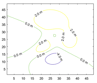
Example: Specify Formatting Operator

Create a contour plot that displays labels with one digit after the decimal point followed by the letter m.

contour(peaks,[-4 0 2],"ShowText",true,"LabelFormat","%0.1f m")

Contour plot with labels that include one digit after the decimal point followed by the letter m

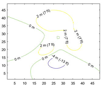
Example: Specify Function Handle

Create a program file called myfun.m and define the following function. The function converts the input from meters to feet and returns a string vector containing each value in meters with the equivalent value in feet in parentheses.

function labels = myfun(vals)
feetPerMeter = 3.28084;
feet = round(vals.*feetPerMeter);
labels = vals + " m (" + feet + " ft)";
labels(vals == 0) = "0 m";
end

Next, create a contour plot and specify the LabelFormat property as a handle to myfun.

contour(peaks,[-4 0 2],"ShowText",true,"LabelFormat",@myfun)

Contour plot with labels that include values in meters and feet

Interval between labeled contour lines, specified as a scalar numeric value. By default, the contour plot includes a label for every contour line when the ShowText property is set to 'on'.

Setting this property sets the associated mode property to manual.

Data Types: single | double | int8 | int16 | int32 | int64 | uint8 | uint16 | uint32 | uint64

Selection mode for the TextStep, specified as one of these values:

  • 'auto' — Determine value based on the ZData values. If the ShowText property is set to 'on', then the contour function labels every contour line.

  • 'manual' — Use a manually specified value. To specify the value, set the TextStep property.

Contour lines to label, specified as a vector of real values.

Setting this property sets the associated mode property to manual.

Data Types: single | double | int8 | int16 | int32 | int64 | uint8 | uint16 | uint32 | uint64

Selection mode for the TextList, specified as one of these values:

  • 'auto' — Use values equal to the values of the LevelList property. The contour plot includes a text label for each line.

  • 'manual' — Use manually specified values. Specify the values by setting the TextList property.

Data

expand all

Contour matrix, returned as a two-row matrix of following form.

Z1, x1,1, x1,2, ..., x1,N1, Z2, x2,1, x2,2, ..., x2,N2, Z3, ...
N1, y1,1, y1,2, ..., y1,N1, N2, y2,1, y2,2, ..., y2,N2, N3, ...

The columns of the matrix define the contour lines. Each contour line starts with a column containing Z and N values:

  • Zi — The height of the ith contour line

  • Ni — The number of vertices in the ith contour line

  • (xij, yij) — The coordinates of the vertices for the ith contour line, where j ranges from 1 to Ni

x values, specified as a vector or matrix.

  • If XData is a vector, then length(XData) must equal size(ZData,2) and YData must also be a vector. The XData values must be strictly increasing or strictly decreasing and cannot contain any duplicates.

  • If XData is a matrix, then size(XData) and size(YData) must equal size(ZData). Typically, you should set the XData values so that the columns are strictly increasing or strictly decreasing and the rows are uniform (or the rows are strictly increasing or strictly decreasing and the columns are uniform).

Setting this property sets the associated mode property to manual.

Data Types: single | double | int8 | int16 | int32 | int64 | uint8 | uint16 | uint32 | uint64 | logical

Selection mode for the XData, specified as one of these values:

  • 'auto' — Set the XData using the column indices of ZData.

  • 'manual' — Use manually specified values. To specify the values, set the XData property directly, or specify the input argument X to the contour, contourf, or contour3 function.

Variable linked to XData, specified as a character vector or string containing a MATLAB workspace variable name. MATLAB evaluates the variable in the base workspace to generate the XData.

By default, there is no linked variable so the value is an empty character vector, ''. If you link a variable, then MATLAB does not update the XData values immediately. To force an update of the data values, use the refreshdata function.

Note

If you change one data source property to a variable that contains data of a different dimension, you might cause the function to generate a warning and not render the graph until you have changed all data source properties to appropriate values.

Example: 'x'

y values, specified as a vector or matrix.

  • If YData is a vector, then length(YData) must equal size(ZData,1) and XData must also be a vector. The XData values must be strictly increasing or strictly decreasing and cannot contain any duplicates.

  • If YData is a matrix, then size(XData) and size(YData) must equal size(ZData). Typically, you should set the YData values so that the columns are strictly increasing or strictly decreasing and the rows are uniform (or the rows are strictly increasing or strictly decreasing and the columns are uniform).

Setting this property sets the associated mode property to manual.

Data Types: single | double | int8 | int16 | int32 | int64 | uint8 | uint16 | uint32 | uint64 | logical

Selection mode for the YData, specified as one of these values:

  • 'auto' — Set the YData using the row indices of ZData.

  • 'manual' — Use manually specified values. To specify the values, set the YData property directly, or specify the input argument Y to the contour, contourf, or contour3 function.

Variable linked to YData, specified as a character vector or string containing a MATLAB workspace variable name. MATLAB evaluates the variable in the base workspace to generate the YData.

By default, there is no linked variable so the value is an empty character vector, ''. If you link a variable, then MATLAB does not update the YData values immediately. To force an update of the data values, use the refreshdata function.

Note

If you change one data source property to a variable that contains data of a different dimension, you might cause the function to generate a warning and not render the graph until you have changed all data source properties to appropriate values.

Example: 'y'

Data that defines the surface to contour, specified as a matrix. ZData must be at least a 2-by-2 matrix.

Setting this property sets the associated mode property to manual.

Data Types: single | double | int8 | int16 | int32 | int64 | uint8 | uint16 | uint32 | uint64

Variable linked to ZData, specified as a character vector or string containing a MATLAB workspace variable name. MATLAB evaluates the variable in the base workspace to generate the ZData.

By default, there is no linked variable so the value is an empty character vector, ''. If you link a variable, then MATLAB does not update the ZData values immediately. To force an update of the data values, use the refreshdata function.

Note

If you change one data source property to a variable that contains data of a different dimension, you might cause the function to generate a warning and not render the graph until you have changed all data source properties to appropriate values.

Example: 'z'

Legend

expand all

Legend label, specified as a character vector or string scalar. The legend does not display until you call the legend command. If you do not specify the text, then legend sets the label using the form 'dataN'.

Include object in the legend, specified as an Annotation object. Set the underlying IconDisplayStyle property of the Annotation object to one of these values:

  • "on" — Include the object in the legend (default).

  • "off" — Do not include the object in the legend.

For example, to exclude the Contour object called obj from the legend, set the IconDisplayStyle property to "off".

obj.Annotation.LegendInformation.IconDisplayStyle = "off";

Alternatively, you can control the items in a legend using the legend function. Specify the first input argument as a vector of the graphics objects to include. If you do not specify an existing graphics object in the first input argument, then it does not appear in the legend. However, graphics objects added to the axes after the legend is created do appear in the legend. Consider creating the legend after creating all the plots to avoid extra items.

Interactivity

expand all

State of visibility, specified as "on" or "off", or as numeric or logical 1 (true) or 0 (false). A value of "on" is equivalent to true, and "off" is equivalent to false. Thus, you can use the value of this property as a logical value. The value is stored as an on/off logical value of type matlab.lang.OnOffSwitchState.

  • "on" — Display the object.

  • "off" — Hide the object without deleting it. You still can access the properties of an invisible object.

Data tip content, specified as a DataTipTemplate object. You can control the content that appears in a data tip by modifying the properties of the underlying DataTipTemplate object. For a list of properties, see DataTipTemplate Properties.

For an example of modifying data tips, see Create Custom Data Tips.

Note

The DataTipTemplate object is not returned by findobj or findall, and it is not copied by copyobj.

Context menu, specified as a ContextMenu object. Use this property to display a context menu when you right-click the object. Create the context menu using the uicontextmenu function.

Note

If the PickableParts property is set to 'none' or if the HitTest property is set to 'off', then the context menu does not appear.

Selection state, specified as 'on' or 'off', or as numeric or logical 1 (true) or 0 (false). A value of 'on' is equivalent to true, and 'off' is equivalent to false. Thus, you can use the value of this property as a logical value. The value is stored as an on/off logical value of type matlab.lang.OnOffSwitchState.

  • 'on' — Selected. If you click the object when in plot edit mode, then MATLAB sets its Selected property to 'on'. If the SelectionHighlight property also is set to 'on', then MATLAB displays selection handles around the object.

  • 'off' — Not selected.

Display of selection handles when selected, specified as 'on' or 'off', or as numeric or logical 1 (true) or 0 (false). A value of 'on' is equivalent to true, and 'off' is equivalent to false. Thus, you can use the value of this property as a logical value. The value is stored as an on/off logical value of type matlab.lang.OnOffSwitchState.

  • 'on' — Display selection handles when the Selected property is set to 'on'.

  • 'off' — Never display selection handles, even when the Selected property is set to 'on'.

Clipping of the object to the axes limits, specified as 'on' or 'off', or as numeric or logical 1 (true) or 0 (false). A value of 'on' is equivalent to true, and 'off' is equivalent to false. Thus, you can use the value of this property as a logical value. The value is stored as an on/off logical value of type matlab.lang.OnOffSwitchState.

  • A value of 'on' clips parts of the object that are outside the axes limits.

  • A value of 'off' displays the entire object, even if parts of it appear outside the axes limits. Parts of the object might appear outside the axes limits if you create a plot, set hold on, freeze the axis scaling, and then create the object so that it is larger than the original plot.

The Clipping property of the axes that contains the object must be set to 'on'. Otherwise, this property has no effect. For more information about the clipping behavior, see the Clipping property of the axes.

Callbacks

expand all

Mouse-click callback, specified as one of these values:

  • Function handle

  • Cell array containing a function handle and additional arguments

  • Character vector that is a valid MATLAB command or function, which is evaluated in the base workspace (not recommended)

Use this property to execute code when you click the object. If you specify this property using a function handle, then MATLAB passes two arguments to the callback function when executing the callback:

  • Clicked object — Access properties of the clicked object from within the callback function.

  • Event data — Empty argument. Replace it with the tilde character (~) in the function definition to indicate that this argument is not used.

For more information on how to use function handles to define callback functions, see Create Callbacks for Graphics Objects.

Note

If the PickableParts property is set to 'none' or if the HitTest property is set to 'off', then this callback does not execute.

Object creation function, specified as one of these values:

  • Function handle.

  • Cell array in which the first element is a function handle. Subsequent elements in the cell array are the arguments to pass to the callback function.

  • Character vector containing a valid MATLAB expression (not recommended). MATLAB evaluates this expression in the base workspace.

For more information about specifying a callback as a function handle, cell array, or character vector, see Create Callbacks for Graphics Objects.

This property specifies a callback function to execute when MATLAB creates the object. MATLAB initializes all property values before executing the CreateFcn callback. If you do not specify the CreateFcn property, then MATLAB executes a default creation function.

Setting the CreateFcn property on an existing component has no effect.

If you specify this property as a function handle or cell array, you can access the object that is being created using the first argument of the callback function. Otherwise, use the gcbo function to access the object.

Object deletion function, specified as one of these values:

  • Function handle.

  • Cell array in which the first element is a function handle. Subsequent elements in the cell array are the arguments to pass to the callback function.

  • Character vector containing a valid MATLAB expression (not recommended). MATLAB evaluates this expression in the base workspace.

For more information about specifying a callback as a function handle, cell array, or character vector, see Create Callbacks for Graphics Objects.

This property specifies a callback function to execute when MATLAB deletes the object. MATLAB executes the DeleteFcn callback before destroying the properties of the object. If you do not specify the DeleteFcn property, then MATLAB executes a default deletion function.

If you specify this property as a function handle or cell array, you can access the object that is being deleted using the first argument of the callback function. Otherwise, use the gcbo function to access the object.

Callback Execution Control

expand all

Callback interruption, specified as 'on' or 'off', or as numeric or logical 1 (true) or 0 (false). A value of 'on' is equivalent to true, and 'off' is equivalent to false. Thus, you can use the value of this property as a logical value. The value is stored as an on/off logical value of type matlab.lang.OnOffSwitchState.

This property determines if a running callback can be interrupted. There are two callback states to consider:

  • The running callback is the currently executing callback.

  • The interrupting callback is a callback that tries to interrupt the running callback.

MATLAB determines callback interruption behavior whenever it executes a command that processes the callback queue. These commands include drawnow, figure, uifigure, getframe, waitfor, and pause.

If the running callback does not contain one of these commands, then no interruption occurs. MATLAB first finishes executing the running callback, and later executes the interrupting callback.

If the running callback does contain one of these commands, then the Interruptible property of the object that owns the running callback determines if the interruption occurs:

  • If the value of Interruptible is 'off', then no interruption occurs. Instead, the BusyAction property of the object that owns the interrupting callback determines if the interrupting callback is discarded or added to the callback queue.

  • If the value of Interruptible is 'on', then the interruption occurs. The next time MATLAB processes the callback queue, it stops the execution of the running callback and executes the interrupting callback. After the interrupting callback completes, MATLAB then resumes executing the running callback.

Note

Callback interruption and execution behave differently in these situations:

  • If the interrupting callback is a DeleteFcn, CloseRequestFcn, or SizeChangedFcn callback, then the interruption occurs regardless of the Interruptible property value.

  • If the running callback is currently executing the waitfor function, then the interruption occurs regardless of the Interruptible property value.

  • If the interrupting callback is owned by a Timer object, then the callback executes according to schedule regardless of the Interruptible property value.

Note

When an interruption occurs, MATLAB does not save the state of properties or the display. For example, the object returned by the gca or gcf command might change when another callback executes.

Callback queuing, specified as 'queue' or 'cancel'. The BusyAction property determines how MATLAB handles the execution of interrupting callbacks. There are two callback states to consider:

  • The running callback is the currently executing callback.

  • The interrupting callback is a callback that tries to interrupt the running callback.

The BusyAction property determines callback queuing behavior only when both of these conditions are met:

  • The running callback contains a command that processes the callback queue, such as drawnow, figure, uifigure, getframe, waitfor, or pause.

  • The value of the Interruptible property of the object that owns the running callback is 'off'.

Under these conditions, the BusyAction property of the object that owns the interrupting callback determines how MATLAB handles the interrupting callback. These are possible values of the BusyAction property:

  • 'queue' — Puts the interrupting callback in a queue to be processed after the running callback finishes execution.

  • 'cancel' — Does not execute the interrupting callback.

Ability to capture mouse clicks, specified as one of these values:

  • 'visible' — Capture mouse clicks only when visible. The Visible property must be set to 'on'. The HitTest property determines if the Contour object responds to the click or if an ancestor does.

  • 'none' — Cannot capture mouse clicks. Clicking the Contour object passes the click to the object behind it in the current view of the figure window. The HitTest property of the Contour object has no effect.

Response to captured mouse clicks, specified as 'on' or 'off', or as numeric or logical 1 (true) or 0 (false). A value of 'on' is equivalent to true, and 'off' is equivalent to false. Thus, you can use the value of this property as a logical value. The value is stored as an on/off logical value of type matlab.lang.OnOffSwitchState.

  • 'on' — Trigger the ButtonDownFcn callback of the Contour object. If you have defined the ContextMenu property, then invoke the context menu.

  • 'off' — Trigger the callbacks for the nearest ancestor of the Contour object that has one of these:

    • HitTest property set to 'on'

    • PickableParts property set to a value that enables the ancestor to capture mouse clicks

Note

The PickableParts property determines if the Contour object can capture mouse clicks. If it cannot, then the HitTest property has no effect.

This property is read-only.

Deletion status, returned as an on/off logical value of type matlab.lang.OnOffSwitchState.

MATLAB sets the BeingDeleted property to 'on' when the DeleteFcn callback begins execution. The BeingDeleted property remains set to 'on' until the component object no longer exists.

Check the value of the BeingDeleted property to verify that the object is not about to be deleted before querying or modifying it.

Parent/Child

expand all

Parent, specified as an Axes, Group, or Transform object.

Children, returned as an empty GraphicsPlaceholder array or a DataTip object array. Use this property to view a list of data tips that are plotted on the chart.

You cannot add or remove children using the Children property. To add a child to this list, set the Parent property of the DataTip object to the chart object.

Visibility of the object handle in the Children property of the parent, specified as one of these values:

  • "on" — Object handle is always visible.

  • "off" — Object handle is invisible at all times. This option is useful for preventing unintended changes by another function. Set the HandleVisibility to "off" to temporarily hide the handle during the execution of that function.

  • "callback" — Object handle is visible from within callbacks or functions invoked by callbacks, but not from within functions invoked from the command line. This option blocks access to the object at the command line, but permits callback functions to access it.

If the object is not listed in the Children property of the parent, then functions that obtain object handles by searching the object hierarchy or querying handle properties cannot return it. Examples of such functions include the get, findobj, gca, gcf, gco, newplot, cla, clf, and close functions.

Hidden object handles are still valid. Set the root ShowHiddenHandles property to "on" to list all object handles regardless of their HandleVisibility property setting.

Identifiers

expand all

This property is read-only.

Type of graphics object, returned as 'contour'.

Object identifier, specified as a character vector or string scalar. You can specify a unique Tag value to serve as an identifier for an object. When you need access to the object elsewhere in your code, you can use the findobj function to search for the object based on the Tag value.

User data, specified as any MATLAB array. For example, you can specify a scalar, vector, matrix, cell array, character array, table, or structure. Use this property to store arbitrary data on an object.

If you are working in App Designer, create public or private properties in the app to share data instead of using the UserData property. For more information, see Share Data Within App Designer Apps.

Version History

Introduced before R2006a

expand all