Find Regions in Spatially Referenced Multispectral Image
This example shows how to identify water and vegetation regions in a Landsat 8 multispectral image and spatially reference the image.
This example requires the Hyperspectral Imaging Library for Image Processing Toolbox™. You can install the Hyperspectral Imaging Library for Image Processing Toolbox from Add-On Explorer. For more information about installing add-ons, see Get and Manage Add-Ons. The Hyperspectral Imaging Library for Image Processing Toolbox requires desktop MATLAB®, as MATLAB® Online™ and MATLAB® Mobile™ do not support the library.
Spectral indices characterize the specific features of interest of a target using its biophysical and chemical properties. These features of interest enable you to identify plant, water, and soil regions, as well as various forms of built-up regions. This example uses modified normalized difference water index (MNDWI) and green vegetation index (GVI) spectral indices to identify water and vegetation regions respectively. For more information on spectral indices, see Spectral Indices.
Load and Visualize Multispectral Data
Landsat 8 is an Earth observation satellite that carries the Operational Land Imager (OLI) and Thermal Infrared Sensor (TIRS) instruments.
Download the Landsat 8 data set. The data set has 11 spectral bands with wavelengths that range from 440 nm to 2200 nm.
Download the data set and unzip the file by using the downloadLandsat8Dataset helper function. This function is attached to the example as a supporting file.
zipfile = "LC08_L1TP_113082_20211206_20211215_02_T1.zip";
landsat8Data_url = "https://ssd.mathworks.com/supportfiles/image/data/" + zipfile;
downloadLandsat8Dataset(landsat8Data_url,pwd)
Downloading the Landsat 8 OLI dataset.
This can take several minutes to download...
Done.
Read the Landsat 8 multispectral data into the workspace.
filepath = fullfile("LC08_L1TP_113082_20211206_20211215_02_T1","LC08_L1TP_113082_20211206_20211215_02_T1_MTL.txt");
mcube = geomulticube(filepath);
Estimate an RGB image from the data cube by using colorize function.
rgbImg = colorize(mcube);
Adjust image intensity values using the imadjustn function for better visualization.
rgbImg = imadjustn(rgbImg);
Display the RGB image of the test data. Notice that without spatial referencing, this figure does not provide any geographic information.
figure
imshow(rgbImg)
title("RGB Image of Data Cube")
Display Area of Interest on a Map
The Landsat 8 data set contains a GeoTIFF file. Obtain information about the GeoTIFF file.
filename = fullfile("LC08_L1TP_113082_20211206_20211215_02_T1","LC08_L1TP_113082_20211206_20211215_02_T1_B1.TIF");
info = georasterinfo(filename);
Get the map raster reference object. The reference object contains information such as the x-y world limits.
R = info.RasterReference;
Create a rectangular area of interest by using the aoiquad (Mapping Toolbox) function. The function represents the AOI using a polygon shape object in projected coordinates.
dataRegion = aoiquad(R);
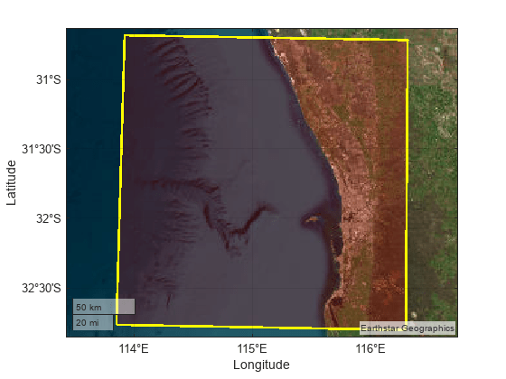
Plot the region of interest using satellite imagery.
figure
geoplot(dataRegion, ...
    LineWidth=2, ...
    EdgeColor="yellow", ...
    FaceColor="red", ...
    FaceAlpha=0.2)
hold on
geobasemap satellite

Import the shapefile worldcities.shp, which contains geographic information about major world cities as a geospatial table, by using the readgeotable (Mapping Toolbox) function. A geospatial table is a table or timetable object that contains a Shape variable and attribute variables. For more information on geospatial tables, see Create Geospatial Tables (Mapping Toolbox). You can also use the worldrivers.shp and worldlakes.shp shapefiles to display major world rivers and lakes, respectively.
cities = readgeotable("worldcities.shp");Query the test data to determine which major cities are within the geographic extent of the rectangular data region. The data region contains a single city from the worldcities.shp geospatial table.
[citiesX,citiesY] = projfwd(R.ProjectedCRS,cities.Shape.Latitude,cities.Shape.Longitude);
citiesMapShape = mappointshape(citiesX,citiesY);
citiesMapShape.ProjectedCRS = R.ProjectedCRS;
inRegion = isinterior(dataRegion,citiesMapShape);
citiesInRegion = cities(inRegion,:);
Plot and label the major city in the area of interest.
geoplot(citiesInRegion, ...
    MarkerSize=14)
text(citiesInRegion.Shape.Latitude+0.07,citiesInRegion.Shape.Longitude+0.03,citiesInRegion.Name, ...
    HorizontalAlignment="left", ...
    FontWeight="bold", ...
    FontSize=14, ...
    Color=[1 1 1])
title("Geographic Extent of Landsat 8 Multispectal Image")

Find Water and Vegetation Regions in the Image
Compute the spectral index value for each pixel in the data cube by using spectralIndices function. Use the MNDWI and GVI to detect water and green vegetation regions, respectively.
indices = spectralIndices(mcube,["MNDWI","GVI"]);
Water regions typically have MNDWI values greater than 0. Vegetation regions typically have GVI values greater than 1. Specify the threshold values for performing thresholding of the MNDWI and GVI images to segment the water and green vegetation regions.
threshold = [0 1];
Generate binary images with a value of 1 for pixels with a score greater than the specified thresholds. All other pixels have a value of 0. The regions in the MNDWI and GVI binary images with a value of 1 correspond to the water and green vegetation regions, respectively.
Overlay the binary images on the RGB image by using labeloverlay function.
overlayImg = rgbImg;
labelColor = [0 0 1; 0 1 0];
for num = 1:numel(indices)
    indexMap = indices(num).IndexImage;
    thIndexMap = indexMap > threshold(num);
    overlayImg = labeloverlay(overlayImg,thIndexMap,Colormap=labelColor(num,:),Transparency=0.5);
end
Resize the overlaid RGB image by using the mapresize (Mapping Toolbox) function. For this example, reduce the size of the overlaid RGB image to one fourth of the original size.
scale = 1/4;
[reducedOverlayImg,reducedR] = mapresize(overlayImg,R,scale);
Calculate the latitude-longitude limits of the image.
[xlimits,ylimits] = bounds(dataRegion);
[latLimits,lonLimits] = projinv(dataRegion.ProjectedCRS,xlimits,ylimits);
Display the overlaid image on a map. The axes displays the water regions in blue and the green vegetation regions in green.
mstruct = defaultm("tranmerc");
mstruct.origin = [0 R.ProjectedCRS.ProjectionParameters.LongitudeOfNaturalOrigin];
mstruct.geoid = R.ProjectedCRS.GeographicCRS.Spheroid;
mstruct.scalefactor = R.ProjectedCRS.ProjectionParameters.ScaleFactorAtNaturalOrigin;
mstruct.falseeasting = R.ProjectedCRS.ProjectionParameters.FalseEasting;
mstruct = defaultm(mstruct);

figure
ax = axesm(mstruct,Grid="on", ...
    GColor=[1 1 1],GLineStyle="-", ...
    MapLatlimit=latLimits,MapLonLimit=lonLimits, ...
    ParallelLabel="on",PLabelLocation=0.5,PLabelMeridian="west", ...
    MeridianLabel="on",MLabelLocation=0.75,MLabelParallel="south", ...
    MLabelRound=-1,PLabelRound=-1, ...
    PLineVisible="on",PLineLocation=0.5, ...
    MLineVisible="on",MlineLocation=0.75);
[X,Y] = worldGrid(reducedR);
mapshow(X,Y,reducedOverlayImg)
axis off
dim = [0.77 0.5 0.3 0.3];
annotation(textbox=dim,String="Water Bodies", ...
    Color=[1 1 1], ...
    BackgroundColor=[0 0 1], ...
    FaceAlpha=0.5, ...
    FitBoxToText="on")
dim = [0.77 0.4 0.3 0.3];
annotation(textbox=dim,String="Green Vegetation", ...
    BackgroundColor=[0 1 0], ...
    FaceAlpha=0.5, ...
    FitBoxToText="on")
title("Water and Vegetation Region of Spatially Referenced Image")

See Also
multicube | geomulticube | spectralIndices | colorize | geotiffinfo (Mapping Toolbox) | geoplot (Mapping Toolbox) | mapshow (Mapping Toolbox)