pzplot
Pole-zero plot of dynamic system model with additional plot customization options
Syntax
Description
pzplot lets you plot pole-zero maps with a broader range of
plot customization options than pzmap. You can use
pzplot to obtain the plot handle and use it to customize the
plot, such as modify the axes labels, limits and units. You can also use
pzplot to draw a pole-zero plot on an existing set of axes
represented by an axes handle. To customize an existing plot using the plot
handle:
Obtain the plot handle
Use
getoptionsto obtain the option setUpdate the plot using
setoptionsto modify the required options
For more information, see Customizing Response Plots from the Command Line (Control System Toolbox). To create pole-zero maps with default options or to extract pole-zero data, use
pzmap.
h = pzplot(sys)sys and returns the plot handle h to the
plot. x and o indicates poles and zeros
respectively.
h = pzplot(...,plotoptions)plotoptions. For more information on the ways to change
properties of your plots, see Ways to Customize Plots (Control System Toolbox).
Examples
Pole-Zero Plot with Custom Plot Title
Plot the poles and zeros of the continuous-time system represented by the following transfer function:
sys = tf([2 5 1],[1 3 5]);
h = pzplot(sys);
grid on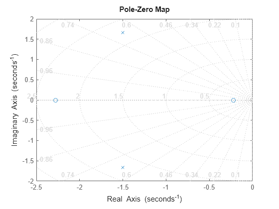
Turning on the grid displays lines of constant damping ratio (zeta) and lines of constant natural frequency (wn). This system has two real zeros, marked by o on the plot. The system also has a pair of complex poles, marked by x.
Change the color of the plot title. To do so, use the plot handle, h.
p = getoptions(h);
p.Title.Color = [1,0,0];
setoptions(h,p);
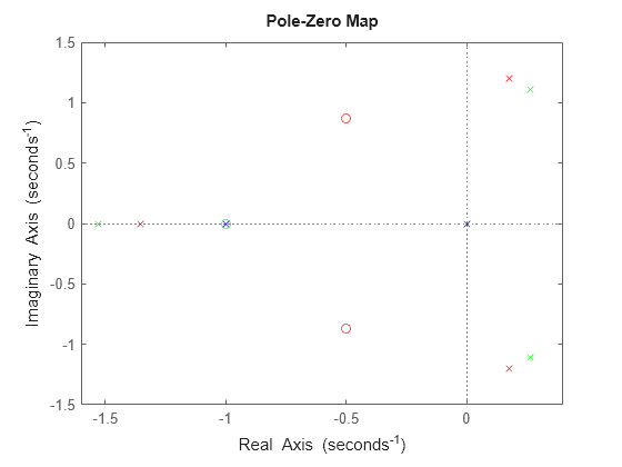
Pole-Zero Plot of Multiple Models
For this example, load a 3-by-1 array of transfer function models.
load('tfArrayMargin.mat','sys');
size(sys)
3x1 array of transfer functions.
Each model has 1 outputs and 1 inputs.
Plot the poles and zeros of the model array. Define the colors for each model. For this example, use red for the first model, green for the second and blue for the third model in the array.
pzplot(sys(:,:,1),'r',sys(:,:,2),'g',sys(:,:,3),'b');
Pole-Zero Plot with Custom Options
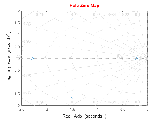
Plot the poles and zeros of the continuous-time system represented by the following transfer function with a custom option set:
Create the custom option set using pzoptions.
plotoptions = pzoptions;
For this example, specify the grid to be visible.
plotoptions.Grid = 'on';Use the specified options to create a pole-zero map of the transfer function.
h = pzplot(tf([2 5 1],[1 3 5]),plotoptions);
![]()
Turning on the grid displays lines of constant damping ratio (zeta) and lines of constant natural frequency (wn). This system has two real zeros, marked by o on the plot. The system also has a pair of complex poles, marked by x.
Input Arguments
Output Arguments
Tips
Version History
Introduced before R2006a
See Also
getoptions | pzmap | setoptions | iopzplot | pzoptions
Topics
- Ways to Customize Plots (Control System Toolbox)
You can also select a web site from the following list:
Americas
- América Latina (Español)
- Canada (English)
- United States (English)
Europe
- Belgium (English)
- Denmark (English)
- Deutschland (Deutsch)
- España (Español)
- Finland (English)
- France (Français)
- Ireland (English)
- Italia (Italiano)
- Luxembourg (English)
- Netherlands (English)
- Norway (English)
- Österreich (Deutsch)
- Portugal (English)
- Sweden (English)
- Switzerland
- United Kingdom (English)