Customize Linear Analysis Plots at Command Line
When creating linear analysis plots, you can programmatically edit the appearance and behavior of the plots. Customizing the response properties allows you to:
Efficiently customize a large number of plots in a batch analysis process.
Add response plots to a UI and update plot appearance based on user input.
To programmatically customize your response plot, you can use one of these approaches.
Customize response at creation — Specify one or more name-value arguments when creating the plot. Use this method for relatively simple changes to the plot appearance. (since R2026a)
Customize response after creation — Return a chart object and modify its properties using dot notation. Use this method for more complex customizations.
You can also interactively modify individual response plot properties using the:
Property Editor — For more information, see Customize Linear Analysis Plots Using Property Editor.
Customize Response At Creation
Since R2026a
To programmatically customize response plots at the time of creation, you can specify one or more name-value arguments for these plotting functions.
Plot Type | Plot Function |
|---|---|
Bode magnitude and phase | bodeplot |
Impulse response | impulseplot |
Initial condition | initialplot |
Pole/zero maps for input/output pairs | iopzplot |
Time response to arbitrary inputs | lsimplot |
Nichols chart | nicholsplot |
Nyquist | nyquistplot |
Pole/zero | pzplot |
Root locus | rlocusplot |
Singular values of the frequency response | sigmaplot |
Step response | stepplot |
For more information on specifying name-value arguments for a response plot, see the corresponding plot function page. Using name-value arguments, you can specify response properties such as:
Name
Color
Visibility
Line style and weight
Marker style and size
You can specify some response properties, such as those for color and line style, by using input arguments or name-value arguments. If you specify a property using both an input argument and a name-value argument, the name-value argument takes precedence.
When plotting responses for multiple systems, any name-value arguments that you specify apply to all the responses.
Customize Response After Creation
To programmatically customize response plots after creation, you must return a chart object when calling one of these plotting functions. You can modify the plot appearance and behavior by modifying the chart object properties.
Plot Type | Plot Function | Chart Object Properties |
|---|---|---|
Bode magnitude and phase | bodeplot | BodePlot Properties |
Impulse response | impulseplot | ImpulsePlot Properties |
Initial condition | initialplot | InitialPlot Properties |
Pole/zero maps for input/output pairs | iopzplot | IOPZPlot Properties |
Time response to arbitrary inputs | lsimplot | LSimPlot Properties |
Nichols chart | nicholsplot | NicholsPlot Properties |
Nyquist | nyquistplot | NyquistPlot Properties |
Pole/zero | pzplot | PZPlot Properties |
Root locus | rlocusplot | RLocusPlot Properties |
Singular values of the frequency response | sigmaplot | SigmaPlot Properties |
Step response | stepplot | StepPlot Properties |
Hankel singular values | HSVPlot Properties |
For more information on specifying properties for a response plot, see the corresponding chart object properties. By modifying these properties, you can customize plot features such as:
Titles and axis label text and font appearance
Axis limits and units
Response appearance, such as line color, style, and weight
Time or frequency vectors
Grid visibility and color
Input and output visibility for MIMO plots
Response characteristics to display, such as rise time or stability margins
You can also add responses to an existing plot using addResponse or
modify the model associated with a response using dot notation.
Customize Linear Analysis Plot Appearance
For relatively simple changes to the appearance of a linear analysis plot, you can specify response properties using one or more name-value arguments. For example, create a step plot for a transfer function model, specifying the line color and width for the response.
sys = tf(4,[1 0.5 4]);
stepplot(sys,Color="black",LineWidth=2)
For some plot customizations, you must return a chart object and modify its properties using dot notation. As an example, create a step plot for the same transfer function model, returning the chart object.
sys = tf(4,[1 0.5 4]);
sp = stepplot(sys,Color="black",LineWidth=2);
Modify the units for the plot. By default, the step response uses the time units of the plotted linear system. For sys, the time unit is seconds. Change the units of the plot to minutes.
sp.TimeUnit = "minutes";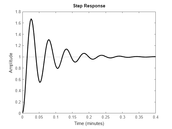
The x-axis label updates to reflect the change of unit. Changing the plot units does not change the time units of the underlying model. To change the model time units, do so before plotting the response.
You can also modify the plot title and axis labels for the plot. For example, change the title text, increase the size of the title font, and make the axes labels to bold.
sp.Title.String = "Step Plot";
sp.Title.FontSize = 16;
sp.XLabel.FontWeight = "bold";
sp.YLabel.FontWeight = "bold";
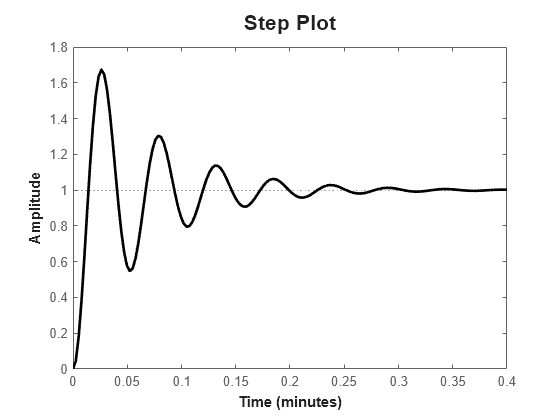
Depending on the plot type, you can configure and display response characteristics in the plot. For example, display the settling time on the step plot.
sp.Characteristics.SettlingTime.Visible = "on";
Modify or Add Linear Model Response
Once you create a response plot, you can modify the properties of the linear system and update the plot. Doing so is helpful for examining the impact of varying model parameters or for updating response plots in a UI based on user input.
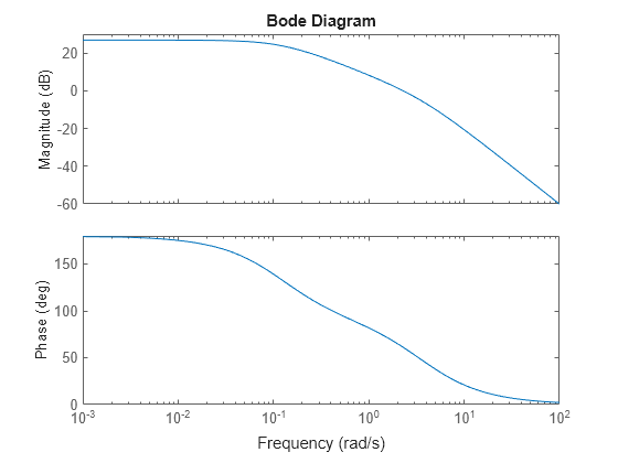
As an example, consider the Bode response for a state-space model.
sys = ss([-4.5 -6;0.6 0.7],[0;-1.5],[-1.1 0],-0.5);
bp = bodeplot(sys);
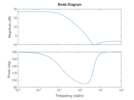
You can modify the linear system for the plot by changing the model for the response. For example, remove the feedthrough component of the plotted state-space model by setting the D matrix to zero.
bp.Responses(1).Model.D = 0;
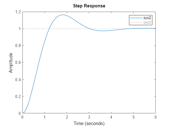
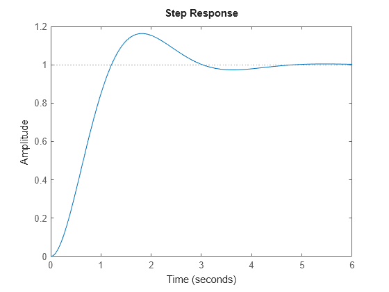
You can also replace the model in a response plot with a new model object. For example, consider a second-order dynamic system with damping ratio zeta.
zeta = 0.5;
wn = 2;
sys2 = tf(wn^2,[1 2*zeta*wn wn^2]);
Plot the step response for this system.
sp = stepplot(sys2);
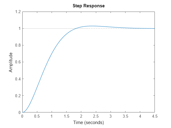
You can update the damping ratio of the model by creating a new transfer function model and replacing the model data.
newZeta = 0.75;
sys3 = tf(wn^2,[1 2*newZeta*wn wn^2]);
sp.Responses.Model = sys3;
You can also add a response to an existing plot using the addResponse function. For example, create a step response for sys2 and subsequently add the response for sys3.
sp2 = stepplot(sys2);
addResponse(sp2,sys3);
legend(Location="southeast")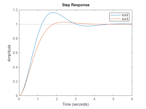
If you have a plot with multiple responses, you can suppress the display of one or more plots without removing the corresponding response from the chart object. For example, hide the second response in the plot.
sp2.Responses(2).Visible = "off";