Main Content

iopzplot

Plot pole-zero map for I/O pairs with additional plot customization options

Description

iopzplot lets you plot pole-zero maps for input/output pairs with a broader range of plot customization options than iopzmap. You can use iopzplot to obtain the plot handle and use it to customize the plot, such as modify the axes labels, limits and units. You can also use iopzplot to draw a pole-zero plot on an existing set of axes represented by an axes handle. To customize an existing plot using the plot handle:

  1. Obtain the plot handle

  2. Use getoptions to obtain the option set

  3. Update the plot using setoptions to modify the required options

For more information, see Customizing Response Plots from the Command Line (Control System Toolbox). To create pole-zero maps with default options or to extract pole-zero data, use iopzmap.

example

h = iopzplot(sys) plots the poles and zeros of each input/output pair of the dynamic system model sys and returns the plot handle h to the plot. x and o indicates poles and zeros respectively.

example

h = iopzplot(sys1,sys2,...,sysN) displays the poles and transmission zeros of multiple models on a single plot. You can specify distinct colors for each model individually.

example

h = iopzplot(sys1,LineSpec1,...,sysN,LineSpecN) sets the line style, marker type, and color for the plot of each system. All systems must have the same number of inputs and outputs to use this syntax.

h = iopzplot(ax,...) plots into the axes specified by ax instead of the current axis gca.

example

h = iopzplot(...,plotoptions) plots the poles and transmission zeros with the options specified in plotoptions. For more information on the ways to change properties of your plots, see Ways to Customize Plots (Control System Toolbox).

Examples

collapse all

Create a pole/zero map of a two-input, two-output dynamic system.

sys = rss(3,2,2);
h = iopzplot(sys);

Figure contains 4 axes objects. Axes object 1 with title From: In(1), ylabel To: Out(1) contains 2 objects of type line. One or more of the lines displays its values using only markers This object represents sys. Axes object 2 with ylabel To: Out(2) contains 2 objects of type line. One or more of the lines displays its values using only markers This object represents sys. Axes object 3 with title From: In(2) contains 2 objects of type line. One or more of the lines displays its values using only markers This object represents sys. Axes object 4 contains 2 objects of type line. One or more of the lines displays its values using only markers This object represents sys.

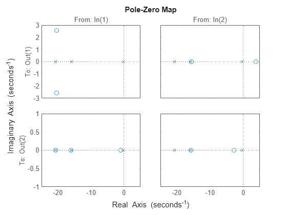
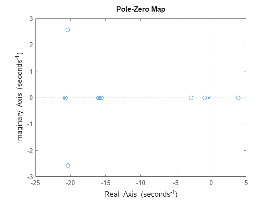
By default, the plot displays the poles and zeros of each I/O pair on its own axis. Use the plot handle to view all I/Os on a single axis.

setoptions(h,'IOGrouping','all')

Figure contains an axes object. The axes object contains 8 objects of type line. One or more of the lines displays its values using only markers These objects represent sys.

View the poles and zeros of a sixth-order state-space model estimated from input-output data. Use the plot handle to display the confidence intervals of the identified model's pole and zero locations.

load iddata1
sys = ssest(z1,6,ssestOptions('focus','simulation'));
h = iopzplot(sys);
showConfidence(h)

Figure contains an axes object. The axes object with title From: u1 To: y1 contains 4 objects of type line. One or more of the lines displays its values using only markers This object represents sys.

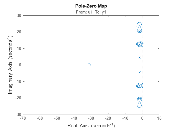
There is at least one pair of complex-conjugate poles whose locations overlap with those of a complex zero, within the 1-σ confidence region. This suggests their redundancy. Hence, a lower (4th) order model might be more robust for the given data.

sys2 = ssest(z1,4,ssestOptions('focus','simulation'));
h = iopzplot(sys,sys2);
showConfidence(h)
legend('6th-order','4th-order')
axis([-20, 10 -30 30])

Figure contains an axes object. The axes object with title From: u1 To: y1 contains 8 objects of type line. One or more of the lines displays its values using only markers These objects represent 6th-order, 4th-order.

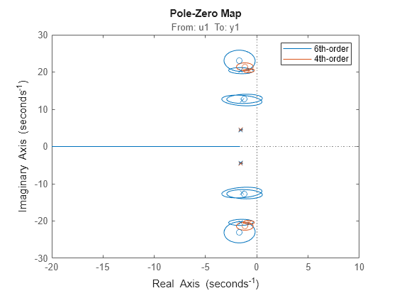
The fourth-order model sys2 shows less variability in the pole-zero locations.

Input Arguments

collapse all

Dynamic system, specified as a SISO or MIMO dynamic system model, or an array of SISO or MIMO dynamic system models. Dynamic systems that you can use include continuous-time or discrete-time numeric LTI models such as tf (Control System Toolbox), zpk (Control System Toolbox), or ss (Control System Toolbox) models.

If sys is a generalized state-space model genss or an uncertain state-space model uss, pzplot returns the poles and transmission zeros of the current or nominal value of sys. If sys is an array of models, pzplot plots the poles and zeros of each model in the array on the same diagram.

Line style, marker, and color, specified as a character vector or string containing symbols. The symbols can appear in any order. You do not need to specify all three characteristics (line style, marker, and color). For example, if you omit the line style and specify the marker, then the plot shows only the marker and no line.

Example: '--or' is a red dashed line with circle markers

Line StyleDescription
-Solid line
--Dashed line
:Dotted line
-.Dash-dot line
MarkerDescription
'o'Circle
'+'Plus sign
'*'Asterisk
'.'Point
'x'Cross
'_'Horizontal line
'|'Vertical line
's'Square
'd'Diamond
'^'Upward-pointing triangle
'v'Downward-pointing triangle
'>'Right-pointing triangle
'<'Left-pointing triangle
'p'Pentagram
'h'Hexagram
ColorDescription

y

yellow

m

magenta

c

cyan

r

red

g

green

b

blue

w

white

k

black

Axes handle, specified as an axes object. If you do not specify the axes object, then pzplot uses the current axes gca to plot the poles and zeros of the system.

Pole-zero plot options, specified as an options object. See pzoptions for a list of available plot options.

Output Arguments

collapse all

Pole-zero plot options handle, returned as a scalar. Use h to query and modify properties of your pole-zero plot. You can use this handle to customize the plot with the getoptions and setoptions commands.

Tips

  • Use sgrid or zgrid to plot lines of constant damping ratio and natural frequency in the s- or z-plane.

Version History

Introduced in R2012a

See Also

| | |

Topics