normalbvarm
Bayesian vector autoregression (VAR) model with normal conjugate prior and fixed covariance for data likelihood
Description
The Bayesian VAR model object normalbvarm specifies the prior distribution of the array of model coefficients Λ in an m-D VAR(p) model, where the innovations covariance matrix Σ is known and fixed. The prior distribution of Λ is the normal conjugate prior model.
In general, when you create a Bayesian VAR model object, it specifies the joint prior distribution and characteristics of the VARX model only. That is, the model object is a template intended for further use. Specifically, to incorporate data into the model for posterior distribution analysis, pass the model object and data to the appropriate object function.
Creation
Description
To create a normalbvarm object, use either the normalbvarm function (described here) or the bayesvarm function. The syntaxes for each function are similar, but the options differ. bayesvarm enables you to set prior hyperparameter values for Minnesota prior[1] regularization easily, whereas normalbvarm requires the entire specification of prior distribution hyperparameters.
PriorMdl = normalbvarm(numseries,numlags)numseries-D Bayesian VAR(numlags) model object PriorMdl, which specifies dimensionalities and prior assumptions for all model coefficients , where:
numseries= m, the number of response time series variables.numlags= p, the AR polynomial order.The prior distribution of λ is the normal conjugate prior model.
The fixed innovations covariance Σ is the m-by-m identity matrix.
PriorMdl = normalbvarm(numseries,numlags,Name,Value)NumSeries and P) using name-value pair arguments. Enclose each property name in quotes. For example, normalbvarm(3,2,'Sigma',4*eye(3),'SeriesNames',["UnemploymentRate" "CPI" "FEDFUNDS"]) specifies the names of the three response variables in the Bayesian VAR(2) model, and fixes the innovations covariance matrix at 4*eye(3).
Input Arguments
Properties
Object Functions
estimate | Estimate posterior distribution of Bayesian vector autoregression (VAR) model parameters |
forecast | Forecast responses from Bayesian vector autoregression (VAR) model |
simsmooth | Simulation smoother of Bayesian vector autoregression (VAR) model |
simulate | Simulate coefficients and innovations covariance matrix of Bayesian vector autoregression (VAR) model |
summarize | Distribution summary statistics of Bayesian vector autoregression (VAR) model |
Examples
Consider the 3-D VAR(4) model for the US inflation (INFL), unemployment (UNRATE), and federal funds (FEDFUNDS) rates.
For all , is a series of independent 3-D normal innovations with a mean of 0 and fixed covariance = , the 3-D identity matrix. Assume that the prior distribution , where is a 39-by-1 vector of means and is the 39-by-39 covariance matrix.
Create a normal conjugate prior model for the 3-D VAR(4) model parameters.
numseries = 3;
numlags = 4;
PriorMdl = normalbvarm(numseries,numlags)
PriorMdl =
  normalbvarm with properties:

        Description: "3-Dimensional VAR(4) Model"
          NumSeries: 3
                  P: 4
        SeriesNames: ["Y1"    "Y2"    "Y3"]
    IncludeConstant: 1
       IncludeTrend: 0
      NumPredictors: 0
                 Mu: [39×1 double]
                  V: [39×39 double]
              Sigma: [3×3 double]
                 AR: {[3×3 double]  [3×3 double]  [3×3 double]  [3×3 double]}
           Constant: [3×1 double]
              Trend: [3×0 double]
               Beta: [3×0 double]
         Covariance: [3×3 double]
PriorMdl is a normalbvarm Bayesian VAR model object representing the prior distribution of the coefficients of the 3-D VAR(4) model. The command line display shows properties of the model. You can display properties by using dot notation.
Display the prior mean matrices of the four AR coefficients by setting each matrix in the cell to a variable.
AR1 = PriorMdl.AR{1}AR1 = 3×3
0 0 0
0 0 0
0 0 0
AR2 = PriorMdl.AR{2}AR2 = 3×3
0 0 0
0 0 0
0 0 0
AR3 = PriorMdl.AR{3}AR3 = 3×3
0 0 0
0 0 0
0 0 0
AR4 = PriorMdl.AR{4}AR4 = 3×3
0 0 0
0 0 0
0 0 0
normalbvarm centers all AR coefficients at 0 by default. The AR property is read only, but it is derived from the writeable property Mu.
Display the fixed innovations covariance .
PriorMdl.Covariance
ans = 3×3

     1     0     0
     0     1     0
     0     0     1
Covariance is a read-only property. To set the value , use the 'Sigma' name-value pair argument or specify the Sigma property by using dot notation. For example:
PriorMdl.Sigma = 4*eye(PriorMdl.NumSeries);
Consider the 3-D VAR(4) model of Create Normal Conjugate Prior Model.
Suppose econometric theory dictates that
Create a normal conjugate prior model for the VAR model coefficients. Specify the value of .
numseries = 3;
numlags = 4;
Sigma = [10e-5 0 10e-4; 0 0.1 -0.2; 10e-4 -0.2 1.6];

PriorMdl = normalbvarm(numseries,numlags,'Sigma',Sigma)
PriorMdl =
normalbvarm with properties:
Description: "3-Dimensional VAR(4) Model"
NumSeries: 3
P: 4
SeriesNames: ["Y1" "Y2" "Y3"]
IncludeConstant: 1
IncludeTrend: 0
NumPredictors: 0
Mu: [39×1 double]
V: [39×39 double]
Sigma: [3×3 double]
AR: {[3×3 double] [3×3 double] [3×3 double] [3×3 double]}
Constant: [3×1 double]
Trend: [3×0 double]
Beta: [3×0 double]
Covariance: [3×3 double]
Because is fixed for normalbvarm prior models, PriorMdl.Sigma and PriorMdl.Covariance are equal.
PriorMdl.Sigma
ans = 3×3

    0.0001         0    0.0010
         0    0.1000   -0.2000
    0.0010   -0.2000    1.6000
PriorMdl.Covariance
ans = 3×3

    0.0001         0    0.0010
         0    0.1000   -0.2000
    0.0010   -0.2000    1.6000
Consider a 1-D Bayesian AR(2) model for the daily NASDAQ returns from January 2, 1990 through December 31, 2001.
The coefficient prior distribution is , where is a 3-by-1 vector of coefficient means and is a 3-by-3 covariance matrix. Assume Var() is 2.
Create a normal conjugate prior model for the AR(2) model parameters.
numseries = 1;
numlags = 2;
PriorMdl = normalbvarm(numseries,numlags,'Sigma',2)
PriorMdl =
normalbvarm with properties:
Description: "1-Dimensional VAR(2) Model"
NumSeries: 1
P: 2
SeriesNames: "Y1"
IncludeConstant: 1
IncludeTrend: 0
NumPredictors: 0
Mu: [3×1 double]
V: [3×3 double]
Sigma: 2
AR: {[0] [0]}
Constant: 0
Trend: [1×0 double]
Beta: [1×0 double]
Covariance: 2
In the 3-D VAR(4) model of Create Normal Conjugate Prior Model, consider excluding lags 2 and 3 from the model.
You cannot exclude coefficient matrices from models, but you can specify high prior tightness on zero for coefficients that you want to exclude.
Create a normal conjugate prior model for the 3-D VAR(4) model parameters. Specify response variable names.
By default, AR coefficient prior means are zero. Specify high tightness values for lags 2 and 3 by setting their prior variances to 1e-6. Leave all other coefficient tightness values at their defaults:
1for AR coefficient variances1e3for constant vector variances0for all coefficient covariances
numseries = 3;
numlags = 4;
seriesnames = ["INFL"; "UNRATE"; "FEDFUNDS"];
vPhi1 = ones(numseries,numseries);
vPhi2 = 1e-6*ones(numseries,numseries);
vPhi3 = 1e-6*ones(numseries,numseries);
vPhi4 = ones(numseries,numseries);
vc = 1e3*ones(3,1);
Vmat = [vPhi1 vPhi2 vPhi3 vPhi4 vc]';
V = diag(Vmat(:));
PriorMdl = normalbvarm(numseries,numlags,'SeriesNames',seriesnames,...
    'V',V)
PriorMdl =
  normalbvarm with properties:

        Description: "3-Dimensional VAR(4) Model"
          NumSeries: 3
                  P: 4
        SeriesNames: ["INFL"    "UNRATE"    "FEDFUNDS"]
    IncludeConstant: 1
       IncludeTrend: 0
      NumPredictors: 0
                 Mu: [39×1 double]
                  V: [39×39 double]
              Sigma: [3×3 double]
                 AR: {[3×3 double]  [3×3 double]  [3×3 double]  [3×3 double]}
           Constant: [3×1 double]
              Trend: [3×0 double]
               Beta: [3×0 double]
         Covariance: [3×3 double]
normalbvarm options enable you to specify coefficient prior hyperparameter values directly, but bayesvarm options are well suited for tuning hyperparameters following the Minnesota regularization method.
Consider the 3-D VAR(4) model of Create Normal Conjugate Prior Model. The model contains 39 coefficients. For coefficient sparsity, create a normal conjugate Bayesian VAR model by using bayesvarm. Specify the following, a priori:
Each response is an AR(1) model, on average, with lag 1 coefficient 0.75.
Prior self-lag coefficients have variance 100. This large variance setting allows the data to influence the posterior more than the prior.
Prior cross-lag coefficients have variance 1. This small variance setting tightens the cross-lag coefficients to zero during estimation.
Prior coefficient covariances decay with increasing lag at a rate of 2 (that is, lower lags are more important than higher lags).
The innovations covariance = .
numseries = 3;
numlags = 4;
seriesnames = ["INFL"; "UNRATE"; "FEDFUNDS"];
Sigma = eye(numseries);
PriorMdl = bayesvarm(numseries,numlags,'ModelType','normal','Sigma',Sigma,...
    'Center',0.75,'SelfLag',100,'CrossLag',1,'Decay',2,'SeriesNames',seriesnames)
PriorMdl =
  normalbvarm with properties:

        Description: "3-Dimensional VAR(4) Model"
          NumSeries: 3
                  P: 4
        SeriesNames: ["INFL"    "UNRATE"    "FEDFUNDS"]
    IncludeConstant: 1
       IncludeTrend: 0
      NumPredictors: 0
                 Mu: [39×1 double]
                  V: [39×39 double]
              Sigma: [3×3 double]
                 AR: {[3×3 double]  [3×3 double]  [3×3 double]  [3×3 double]}
           Constant: [3×1 double]
              Trend: [3×0 double]
               Beta: [3×0 double]
         Covariance: [3×3 double]
Display all prior coefficient means.
Phi1 = PriorMdl.AR{1}Phi1 = 3×3
0.7500 0 0
0 0.7500 0
0 0 0.7500
Phi2 = PriorMdl.AR{2}Phi2 = 3×3
0 0 0
0 0 0
0 0 0
Phi3 = PriorMdl.AR{3}Phi3 = 3×3
0 0 0
0 0 0
0 0 0
Phi4 = PriorMdl.AR{4}Phi4 = 3×3
0 0 0
0 0 0
0 0 0
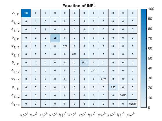
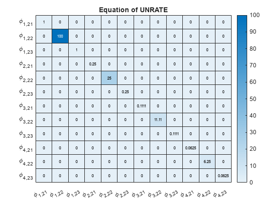
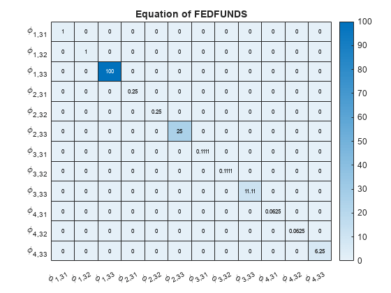
Display a heatmap of the prior coefficient covariances for each response equation.
numexocoeffseqn = PriorMdl.IncludeConstant + ...
    PriorMdl.IncludeTrend + PriorMdl.NumPredictors;             % Number of exogenous coefficients per equation
numcoeffseqn = PriorMdl.NumSeries*PriorMdl.P + numexocoeffseqn; % Total number of coefficients per equation
arcoeffnames = strings(numseries,numlags,numseries);
for j = 1:numseries         % Equations
    for r = 1:numlags
        for k = 1:numseries % Response Variables
            arcoeffnames(k,r,j) = "\phi_{"+r+","+j+k+"}";
        end
    end
    arcoeffseqn = arcoeffnames(:,:,j);
    idx = ((j-1)*numcoeffseqn + 1):(numcoeffseqn*j) - numexocoeffseqn;
    Veqn = PriorMdl.V(idx,idx);
    figure
    heatmap(arcoeffseqn(:),arcoeffseqn(:),Veqn);
    title(sprintf('Equation of %s',seriesnames(j)))
end
Consider the 3-D VAR(4) model of Create Normal Conjugate Prior Model. Estimate the posterior distribution, and generate forecasts from the corresponding posterior predictive distribution.
Load and Preprocess Data
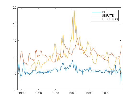
Load the US macroeconomic data set. Compute the inflation rate. Plot all response series.
load Data_USEconModel
seriesnames = ["INFL" "UNRATE" "FEDFUNDS"];
DataTimeTable.INFL = 100*[NaN; price2ret(DataTimeTable.CPIAUCSL)];

figure
plot(DataTimeTable.Time,DataTimeTable{:,seriesnames})
legend(seriesnames)
Stabilize the unemployment and federal funds rates by applying the first difference to each series.
DataTimeTable.DUNRATE = [NaN; diff(DataTimeTable.UNRATE)];
DataTimeTable.DFEDFUNDS = [NaN; diff(DataTimeTable.FEDFUNDS)];
seriesnames(2:3) = "D" + seriesnames(2:3);
Remove all missing values from the data.
rmDataTimeTable = rmmissing(DataTimeTable);
Create Prior Model
Create a normal conjugate Bayesian VAR(4) prior model for the three response series. Specify the response variable names. Assume that the innovations covariance is the identity matrix.
numseries = numel(seriesnames);
numlags = 4;

PriorMdl = normalbvarm(numseries,numlags,'SeriesNames',seriesnames);
Estimate Posterior Distribution
Estimate the posterior distribution by passing the prior model and entire data series to estimate.
PosteriorMdl = estimate(PriorMdl,rmDataTimeTable{:,seriesnames},'Display','equation');Bayesian VAR under normal priors and fixed Sigma
Effective Sample Size: 197
Number of equations: 3
Number of estimated Parameters: 39
VAR Equations
| INFL(-1) DUNRATE(-1) DFEDFUNDS(-1) INFL(-2) DUNRATE(-2) DFEDFUNDS(-2) INFL(-3) DUNRATE(-3) DFEDFUNDS(-3) INFL(-4) DUNRATE(-4) DFEDFUNDS(-4) Constant
------------------------------------------------------------------------------------------------------------------------------------------------------------------------------
INFL | 0.1260 -0.4400 0.1049 0.3176 -0.0545 0.0440 0.4173 0.2421 0.0515 0.0247 -0.1639 0.0080 0.1064
| (0.1367) (0.2673) (0.0700) (0.1551) (0.2854) (0.0739) (0.1536) (0.2811) (0.0766) (0.1605) (0.2652) (0.0708) (0.1483)
DUNRATE | -0.0236 0.4440 0.0350 0.0900 0.2295 0.0520 -0.0330 0.0567 0.0010 0.0298 -0.1665 0.0104 -0.0536
| (0.1367) (0.2673) (0.0700) (0.1551) (0.2854) (0.0739) (0.1536) (0.2811) (0.0766) (0.1605) (0.2652) (0.0708) (0.1483)
DFEDFUNDS | -0.1514 -1.3408 -0.2762 0.3275 -0.2971 -0.3041 0.2609 -0.6971 0.0130 -0.0692 0.1392 -0.1341 -0.3902
| (0.1367) (0.2673) (0.0700) (0.1551) (0.2854) (0.0739) (0.1536) (0.2811) (0.0766) (0.1605) (0.2652) (0.0708) (0.1483)
Innovations Covariance Matrix
| INFL DUNRATE DFEDFUNDS
--------------------------------------
INFL | 1 0 0
| (0) (0) (0)
DUNRATE | 0 1 0
| (0) (0) (0)
DFEDFUNDS | 0 0 1
| (0) (0) (0)
Because the prior is conjugate for the data likelihood, the posterior is analytically tractable. By default, estimate uses the first four observations as a presample to initialize the model.
Generate Forecasts from Posterior Predictive Distribution
From the posterior predictive distribution, generate forecasts over a two-year horizon. Because sampling from the posterior predictive distribution requires the entire data set, specify the prior model in forecast instead of the posterior.
fh = 8;
rng(1); % For reproducibility
FY = forecast(PriorMdl,fh,rmDataTimeTable{:,seriesnames});
FY is an 8-by-3 matrix of forecasts.
Plot the end of the data set and the forecasts.
fp = rmDataTimeTable.Time(end) + calquarters(1:fh);
figure
plotdata = [rmDataTimeTable{end - 10:end,seriesnames}; FY];
plot([rmDataTimeTable.Time(end - 10:end); fp'],plotdata)
hold on
plot([fp(1) fp(1)],ylim,'k-.')
legend(seriesnames)
title('Data and Forecasts')
hold off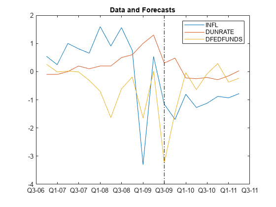
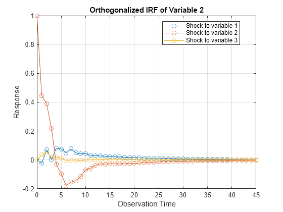
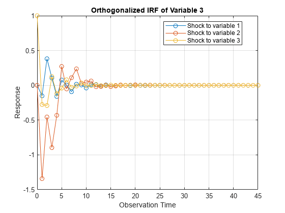
Compute Impulse Responses
Plot impulse response functions by passing posterior estimations to armairf.
armairf(PosteriorMdl.AR,[],'InnovCov',PosteriorMdl.Covariance)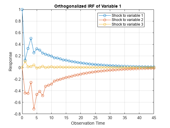
More About
References
[1] Litterman, Robert B. "Forecasting with Bayesian Vector Autoregressions: Five Years of Experience." Journal of Business and Economic Statistics 4, no. 1 (January 1986): 25–38. https://doi.org/10.2307/1391384.
Version History
Introduced in R2020a