forecast

Forecast responses from Bayesian vector autoregression (VAR) model

Since R2020a

Syntax

YF = forecast(PriorMdl,numperiods,Y)

[YF,YFStd] = forecast(PriorMdl,numperiods,Y)

Description

forecast is well suited for computing out-of-sample unconditional forecasts of a Bayesian VAR(p) model that does not contain an exogenous regression component. For advanced applications, such as out-of-sample conditional forecasting, VARX(p) model forecasting, missing value imputation, and Gibbs sampler specification for posterior predictive distribution estimation, see simsmooth.

YF = forecast(PriorMdl,numperiods,Y) returns a path of forecasted responses YF over the length numperiods forecast horizon. Each period in YF is the mean of the posterior predictive distribution, which is derived from the posterior distribution of the prior Bayesian VAR(p) model PriorMdl given the response data Y. The output YF represents the continuation of Y.

NaNs in the data indicate missing values, which forecast removes using list-wise deletion.

[YF,YFStd] = forecast(PriorMdl,numperiods,Y) also returns the corresponding standard deviations of the posterior predictive distribution YFStd.

Examples

Forecast Responses from Posterior Predictive Distribution

Consider the 3-D VAR(4) model for the US inflation (INFL), unemployment (UNRATE), and federal funds (FEDFUNDS) rates.

$$\left[\begin{array}{l}{\text{INFL}}_t\\ {\text{UNRATE}}_t\\ {\text{FEDFUNDS}}_t\end{array}\right]=c+\sum _{j=1}^4{\Phi }_j\left[\begin{array}{l}{\text{INFL}}_{t-j}\\ {\text{UNRATE}}_{t-j}\\ {\text{FEDFUNDS}}_{t-j}\end{array}\right]+\left[\begin{array}{c}{\epsilon }_{1,t}\\ {\epsilon }_{2,t}\\ {\epsilon }_{3,t}\end{array}\right].$$

For all $$t$$, $${\epsilon }_t$$ is a series of independent 3-D normal innovations with a mean of 0 and covariance $\Sigma$. Assume a diffuse prior distribution for the parameters $\left({\left[{\Phi }_1,...,{\Phi }_4,\mathit{c}\right]}^{\prime },\Sigma \right)$.

Load and Preprocess Data

Load the US macroeconomic data set. Compute the inflation rate, stabilize the unemployment and federal funds rates, and remove missing values.

load Data_USEconModel
seriesnames = ["INFL" "UNRATE" "FEDFUNDS"];
DataTimeTable.INFL = 100*[NaN; price2ret(DataTimeTable.CPIAUCSL)];
DataTimeTable.DUNRATE = [NaN; diff(DataTimeTable.UNRATE)];
DataTimeTable.DFEDFUNDS = [NaN; diff(DataTimeTable.FEDFUNDS)];
seriesnames(2:3) = "D" + seriesnames(2:3);
rmDataTimeTable = rmmissing(DataTimeTable);

Create Prior Model

Create a diffuse prior model. Specify the response series names.

numseries = numel(seriesnames);
numlags = 4;

PriorMdl = bayesvarm(numseries,numlags,'SeriesNames',seriesnames);

Forecast Responses

Directly forecast two years (eight quarters) of observations from the posterior predictive distribution. forecast estimates the posterior distribution of the parameters, and then forms the posterior predictive distribution.

numperiods = 8;
YF = forecast(PriorMdl,numperiods,rmDataTimeTable{:,seriesnames});

YF is an 8-by-3 matrix of forecasted responses.

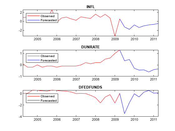
Plot the forecasted responses.

fh = rmDataTimeTable.Time(end) + calquarters(0:8);
tiledlayout(3,1)
for j = 1:PriorMdl.NumSeries
    nexttile
    plot(rmDataTimeTable.Time(end - 20:end),rmDataTimeTable{end - 20:end,seriesnames(j)},'r',...
        fh,[rmDataTimeTable{end,seriesnames(j)}; YF(:,j)],'b');
    legend("Observed","Forecasted",'Location','NorthWest')
    title(seriesnames(j))
end

Estimate Standard Deviations of Posterior Predictive Distribution

Consider the 3-D VAR(4) model of Forecast Responses from Posterior Predictive Distribution.

Load the US macroeconomic data set. Compute the inflation rate, stabilize the unemployment and federal funds rates, and remove missing values.

load Data_USEconModel
seriesnames = ["INFL" "UNRATE" "FEDFUNDS"];
DataTimeTable.INFL = 100*[NaN; price2ret(DataTimeTable.CPIAUCSL)];
DataTimeTable.DUNRATE = [NaN; diff(DataTimeTable.UNRATE)];
DataTimeTable.DFEDFUNDS = [NaN; diff(DataTimeTable.FEDFUNDS)];
seriesnames(2:3) = "D" + seriesnames(2:3);
rmDataTimeTable = rmmissing(DataTimeTable);

Create a diffuse prior model. Specify the response series names.

numseries = numel(seriesnames);
numlags = 4;

PriorMdl = bayesvarm(numseries,numlags,'SeriesNames',seriesnames);

Directly forecast two years (eight quarters) of response observations from the posterior predictive distribution. Return the posterior standard deviations.

numperiods = 8;
[YF,YStd] = forecast(PriorMdl,numperiods,rmDataTimeTable{:,seriesnames});

YF and YStd are 8-by-3 matrices of forecasted responses and corresponding standard deviations, respectively.

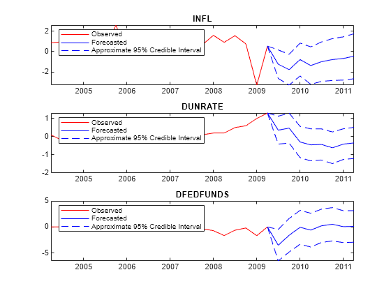
Plot the forecasted responses and approximate 95% credible intervals.

fh = rmDataTimeTable.Time(end) + calquarters(0:8);
for j = 1:PriorMdl.NumSeries
subplot(3,1,j)
plot(rmDataTimeTable.Time(end - 20:end),rmDataTimeTable{end - 20:end,seriesnames(j)},'r',...
    fh,[rmDataTimeTable{end,seriesnames(j)}; YF(:,j)],'b',...
    fh,[rmDataTimeTable{end,seriesnames(j)}; YF(:,j) + 1.96*YStd(:,j)],'b--',...
    fh,[rmDataTimeTable{end,seriesnames(j)}; YF(:,j) - 1.96*YStd(:,j)],'b--');
legend("Observed","Forecasted","Approximate 95% Credible Interval",'Location','NorthWest')
title(seriesnames(j))
end

Input Arguments

PriorMdl — Prior Bayesian VAR model

conjugatebvarm model object | semiconjugatebvarm model object | diffusebvarm model object | normalbvarm model object

Prior Bayesian VAR model, specified as a model object in this table.

Model Object	Description
conjugatebvarm	Dependent, matrix-normal-inverse-Wishart conjugate model returned by bayesvarm, conjugatebvarm, or estimate
semiconjugatebvarm	Independent, normal-inverse-Wishart semiconjugate prior model returned by bayesvarm or semiconjugatebvarm
diffusebvarm	Diffuse prior model returned by bayesvarm or diffusebvarm
normalbvarm	Normal conjugate model with a fixed innovations covariance matrix, returned by bayesvarm, normalbvarm, or estimate

numperiods — Forecast horizon

positive integer

Forecast horizon, or the number of time points in the forecast period, specified as a positive integer.

Data Types: double

Y — Presample and estimation sample multivariate response series

numeric matrix

Presample and estimation sample multivariate response series, specified as a (numlags + numobs)-by-numseries numeric matrix.

Rows correspond to observations, and the last row contains the latest observation. forecast uses the first numlags = PriorMdl.P observations as a presample to initialize the prior model PriorMdl for posterior estimation. forecast estimates the posterior using the remaining numobs observations and PriorMdl.

numseries is the number of response variables PriorMdl.NumSeries. Columns correspond to individual response variables PriorMdl.SeriesNames.

For more details, see Algorithms.

Data Types: double

Output Arguments

YF — Path of multivariate response series forecasts

numeric matrix

Path of multivariate response series forecasts, returned as a numperiods-by-numseries numeric matrix. YF is the mean of the posterior predictive distribution of each period in the forecast horizon.

YF represents the continuation of the response series Y. Rows correspond to observations; row j is the j-period-ahead forecast. Columns correspond to the columns in Y.

YFStd — Forecast standard deviations

numeric matrix

Forecast standard deviations, returned as a numperiods-by-numseries numeric matrix. YFStd is the standard deviation of the posterior predictive distribution of each period in the forecast horizon. Dimensions correspond to the dimensions of YF.

More About

Bayesian Vector Autoregression (VAR) Model

A Bayesian VAR model treats all coefficients and the innovations covariance matrix as random variables in the m-dimensional, stationary VARX(p) model. The model has one of the three forms described in this table.

Model	Equation
Reduced-form VAR(p) in difference-equation notation	$$y_t={\Phi }_1{y}_{t-1}+\mathrm{...}+{\Phi }_p{y}_{t-p}+c+\delta t+{\rm B}{x}_t+{\epsilon }_t.$$
Multivariate regression	$$y_t=Z_t\lambda +{\epsilon }_t.$$
Matrix regression	$$y_t={\Lambda }^{\prime }{z}_t^{\prime }+{\epsilon }_t.$$

For each time t = 1,...,T:

• y_t is the m-dimensional observed response vector, where m = numseries.

• Φ₁,…,Φ_p are the m-by-m AR coefficient matrices of lags 1 through p, where p = numlags.

• c is the m-by-1 vector of model constants if IncludeConstant is true.

• δ is the m-by-1 vector of linear time trend coefficients if IncludeTrend is true.

• Β is the m-by-r matrix of regression coefficients of the r-by-1 vector of observed exogenous predictors x_t, where r = NumPredictors. All predictor variables appear in each equation.

• $$z_t=\left[\begin{array}{ccccccc}{y}_{t-1}^{\prime }& y_{t-2}^{\prime }& \cdots & y_{t-p}^{\prime }& 1& t& x_t^{\prime }\end{array}\right],$$ which is a 1-by-(mp + r + 2) vector, and Z_t is the m-by-m(mp + r + 2) block diagonal matrix

  $$\left[\begin{array}{cccc}{z}_t& 0_z& \cdots & 0_z\\ 0_z& z_t& \cdots & 0_z\\ ⋮& ⋮& \ddots & ⋮\\ 0_z& 0_z& 0_z& z_t\end{array}\right],$$

  where 0_z is a 1-by-(mp + r + 2) vector of zeros.

• $$\Lambda ={\left[\begin{array}{ccccccc}{\Phi }_1& {\Phi }_2& \cdots & {\Phi }_p& c& \delta & {\rm B}\end{array}\right]}^{\prime }$$, which is an (mp + r + 2)-by-m random matrix of the coefficients, and the m(mp + r + 2)-by-1 vector λ = vec(Λ).

• ε_t is an m-by-1 vector of random, serially uncorrelated, multivariate normal innovations with the zero vector for the mean and the m-by-m matrix Σ for the covariance. This assumption implies that the data likelihood is

  $$\ell \left(\Lambda ,\Sigma |y,x\right)={\displaystyle \prod _{t=1}^{T}f\left(y_t;\Lambda ,\Sigma ,z_t\right)},$$

  where f is the m-dimensional multivariate normal density with mean z_tΛ and covariance Σ, evaluated at y_t.

Before considering the data, you impose a joint prior distribution assumption on (Λ,Σ), which is governed by the distribution π(Λ,Σ). In a Bayesian analysis, the distribution of the parameters is updated with information about the parameters obtained from the data likelihood. The result is the joint posterior distribution π(Λ,Σ|Y,X,Y₀), where:

• Y is a T-by-m matrix containing the entire response series {y_t}, t = 1,…,T.

• X is a T-by-m matrix containing the entire exogenous series {x_t}, t = 1,…,T.

• Y₀ is a p-by-m matrix of presample data used to initialize the VAR model for estimation.

Posterior Predictive Distribution

A posterior predictive distribution of a posterior Bayesian VAR(p) model π(Y_f|Y,X) is the distribution of the next τ future response variables after the final observation in the estimation sample Y_f = [y_T+1, y_T+2,…,y_T+τ] given the following, marginalized over Λ and Σ:

• Presample and estimation sample response data Y

• Coefficients Λ

• Innovations covariance matrix Σ

• Estimation and future sample exogenous data X

Symbolically,

$$\pi \left(Y_f|Y,X\right)={\displaystyle \int \pi \left(Y_f|Y,X,\Lambda ,\Sigma \right)\pi \left(\Lambda ,\Sigma |Y,X\right)}d\Lambda d\Sigma .$$

Tips

• Monte Carlo simulation is subject to variation. If forecast uses Monte Carlo simulation, then estimates and inferences might vary when you call forecast multiple times under seemingly equivalent conditions. To reproduce estimation results, set a random number seed by using rng before calling forecast.

Algorithms

• If the posterior predictive distribution is analytically intractable (true for most cases), forecast implements Markov Chain Monte Carlo (MCMC) sampling with Bayesian data augmentation to compute the mean and standard deviation of the posterior predictive distribution. To do so, forecast calls simsmooth, which uses a computationally intensive procedure.

• Most Econometrics Toolbox™ forecast functions accept an estimated or posterior model object from which to generate forecasts. Such a model encompasses the parametric structure and data. However, the forecast function of Bayesian VAR models requires presample and estimation sample data to do the following:

  • Perform Bayesian parameter updating to estimate posterior distributions. forecast implements MCMC sampling with Bayesian data augmentation, which includes a Kalman filter smoothing step that requires the entire observed series.

  • Predict future responses in the presence of two sources of uncertainty:

    • Estimation noise ε₁,…,ε_T, which induces parameter uncertainty

    • Forecast period noise ε_T+1,…,ε_T+numperiods

References

[1] Litterman, Robert B. "Forecasting with Bayesian Vector Autoregressions: Five Years of Experience." Journal of Business and Economic Statistics 4, no. 1 (January 1986): 25–38. https://doi.org/10.2307/1391384.

Version History

Introduced in R2020a