simulate
Simulate posterior draws of Bayesian nonlinear non-Gaussian state-space model parameters
Since R2024b
Syntax
Description
[
returns 1000 random vectors of state-space model parameters Params,accept] = simulate(PriorMdl,Y,params0,Proposal)Params drawn
from the posterior distribution
Π(θ|Y), where
PriorMdl specifies the prior distribution and data likelihood, and
Y is the observed response data. params0 is the
set of initial parameter values and Proposal is the covariance matrix
of the proposal distribution of the Metropolis-Hastings (MH) sampler [9][10] within the Markov chain Monte Carlo
(MCMC) sampler. accept is the acceptance rate of the proposal
draws.
[
specifies options using one or more name-value arguments. For example,
Params,accept] = simulate(PriorMdl,Y,params0,Proposal,Name=Value)simulate(PriorMdl,Y,params0,Proposal,NumDraws=1e3,Thin=4,DoF=10) uses
the multivariate t10 distribution for the MH
proposal, draws 4e3 random vectors of parameters, and thins the sample to
reduce serial correlation by discarding every 3 draws until it retains
1e3 draws.
[
also returns the output Params,accept,Output] = simulate(PriorMdl,Y,params0,Proposal,Name=Value)Output of the custom function that monitors the
MCMC sampler at each iteration, specified by the OutputFunction
name-value argument.
Examples
This example implements an MCMC sampler to random draw parameters from the posterior distribution of the Bayesian nonlinear state-space model in equation. The example uses simulated data.
where the parameters in have the following priors:
, that is, a truncated normal distribution with .
, that is, an inverse gamma distribution with shape and scale .
, that is, a gamma distribution with shape and scale .
To simulate values from posterior distribution, the simulate function requires response data, a bnlssm object that specifies the prior distribution and identifies which parameters to fit to the data, initial values for the parameters, and optionally but a best practice is to provide a carefully tuned proposal distribution moments.
Simulate Series
Consider this data-generating process (DGP).
where the series is a standard Gaussian series of random variables.
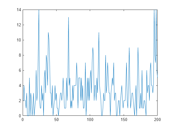
Simulate a series of 200 observations from the process.
rng(1,"twister")    % For reproducibility
T = 200;
thetaDGP = [0.7; 0.2; 3];

numparams = numel(thetaDGP);

MdlXSim = arima(AR=thetaDGP(1),Variance=thetaDGP(2), ...
    Constant=0);
xsim = simulate(MdlXSim,T);
y = random("poisson",thetaDGP(3)*exp(xsim));

figure
plot(y)
Create Bayesian Nonlinear Prior Model
A prior distribution is required to compose a posterior distribution. The Local Functions section contains the functions paramMap and priorDistribution required to specify the Bayesian nonlinear state-space model. The paramMap function specifies the state-space model structure and initial state moments. The priorDistribution function returns the log of the joint prior distribution of the state-space model parameters. You can use the functions only within this script.
Create a Bayesian nonlinear state-space model for the DGP.
Arbitrarily choose values for the hyperparameters.
Indicate that the state-space model observation equation is expressed as a distribution.
To speed up computations, the arguments
AandLogYof theparamMapfunction are written to enable simultaneous evaluation of the transition and observation densities of multiple particles. Specify this characteristic by using theMultipointname-value argument.
% pi(phi,sigma2) hyperparameters
m0 = 0;
v02 = 1;
a0 = 1;
b0 = 1;

% pi(lambda) hyperparameters
alpha0 = 3;
beta0 = 1;

hyperparams = [m0 v02 a0 b0 alpha0 beta0];

PriorMdl = bnlssm(@paramMap,@(x)priorDistribution(x,hyperparams), ...
    ObservationForm="distribution",Multipoint=["A" "LogY"]);
PriorMdl is a bnlssm model specifying the state-space model structure and prior distribution of the state-space model parameters. Because PriorMdl contains unknown values, it serves as a template for posterior simulation with observations.
Choose Initial Parameter Values
Arbitrarily choose a set of initial parameter for the MCMC sampler.
theta0 = [0.5; 0.1; 2];
Tune Proposal Distribution
Obtain optimal proposal distribution moments by passing the prior model, data, and initial parameter values to the tune function.
[params,Proposal] = tune(PriorMdl,y,theta0);
         Optimization and Tuning
      | Params0  Optimized  ProposalStd
----------------------------------------
 c(1) |  0.5000    0.6081      0.1584
 c(2) |  0.1000    0.2190      0.0896
 c(3) |   2        2.8497      0.2166
params and Proposal are the optimized mean and covariance of the Gaussian proposal distribution for the MH sampler used by simulate.
Draw From Posterior Distribution
Simulate the posterior by passing the prior model, simulated data, and optimized proposal moments initial to simulate. Return the draws and the acceptance rate of the MH proposal draws.
[ThetaPostDraws,accept] = simulate(PriorMdl,y,params,Proposal);
[numParams,numDraws] = size(ThetaPostDraws)
numParams =
3
numDraws =
1000
accept
accept =
0.3550
ThetaPostDraws is a 3-by-1000 matrix of random draws from the posterior distribution. By default, simulate treats the first 100 draws as a burn-in sample and excludes them in the results. The acceptance rate is about 42%, which means the MH step of the MCMC sampler retained 42% of the proposed draws from the proposal distribution to represent the posterior distribution.
To diagnose the MCMC sampler, create trace plots of the posterior parameter draws.
paramnames = ["\phi" "\sigma^2" "\lambda"];

figure
h = tiledlayout(3,1);
for j = 1:numParams
    nexttile
    plot(ThetaPostDraws(j,:))
    hold on
    yline(thetaDGP(j))
    ylabel(paramnames(j))
end
title(h,"Posterior Trace Plots")
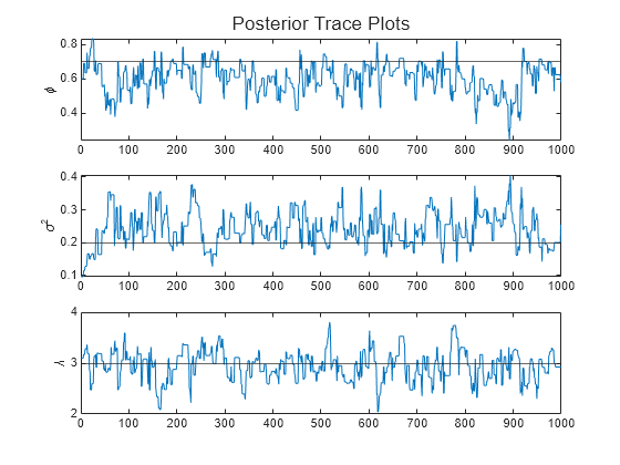
The sampler eventually settles at near the true values of the parameters. In this case, the sample shows serial correlation and transient behavior. You can remedy serial correlation in the sample by adjusting the Thin name-value argument, and you can remedy transient effects by increasing the burn-in period using the BurnIn name-value argument.
Local Functions
These functions specify the state-space model parameter mappings, in distribution form, and the log prior distribution of the parameters.
function [A,B,LogY,Mean0,Cov0,StateType] = paramMap(theta)
    A = theta(1);
    B = sqrt(theta(2));
    LogY = @(y,x)y.*(x + log(theta(3)))- exp(x).*theta(3);
    Mean0 = 0;
    Cov0 = 2;
    StateType = 0;     % Stationary state process
end

function logprior = priorDistribution(theta,hyperparams)
    % Prior of phi
    m0 = hyperparams(1);
    v20 = hyperparams(2);
    pphi = makedist("normal",mu=m0,sigma=sqrt(v20));
    pphi = truncate(pphi,-1,1);
    lpphi = log(pdf(pphi,theta(1)));

    % Prior of sigma2
    a0 = hyperparams(3);
    b0 = hyperparams(4);
    lpsigma2 = -a0*log(b0) - log(gamma(a0)) + (-a0-1)*log(theta(2)) - ...
        1./(b0*theta(2));

    % Prior of lambda
    alpha0 = hyperparams(5);
    beta0 = hyperparams(6);
    plambda = makedist("gamma",alpha0,beta0);
    lplambda = log(pdf(plambda,theta(3)));

    logprior = lpphi + lpsigma2 + lplambda;
end
Consider the model in the example Draw Parameters From Posterior Distribution. Improve the Markov chain convergence by adjusting sampler options.
Create a Bayesian nonlinear state-space model (bnlssm) object that represents the DGP, and then simulate a response path.
rng(1,"twister")    % For reproducibility
T = 200;
thetaDGP = [0.7; 0.2; 3];

numparams = numel(thetaDGP);

MdlXSim = arima(AR=thetaDGP(1),Variance=thetaDGP(2), ...
    Constant=0);
xsim = simulate(MdlXSim,T);
y = random("poisson",thetaDGP(3)*exp(xsim));
Create the Bayesian nonlinear state-space model template for estimation by passing function handles directly to paramMap and paramDistribution to bnlssm (the functions are in Local Functions). Tune the proposal distribution; suppress the tuning algorithm's output.
m0 = 0;
v02 = 1;
a0 = 1;
b0 = 1;
alpha0 = 3;
beta0 = 1;
hyperparams = [m0 v02 a0 b0 alpha0 beta0];

PriorMdl = bnlssm(@paramMap,@(x)priorDistribution(x,hyperparams), ...
    ObservationForm="distribution",Multipoint=["A" "LogY"]);
theta0 = [0.5; 0.1; 2];
[params,Proposal] = tune(PriorMdl,y,theta0,Display="off");
In Draw Parameters From Posterior Distribution:
The optimized proposal moments appear adequate. Therefore, you might not need to adjust the proposal tuning procedure.
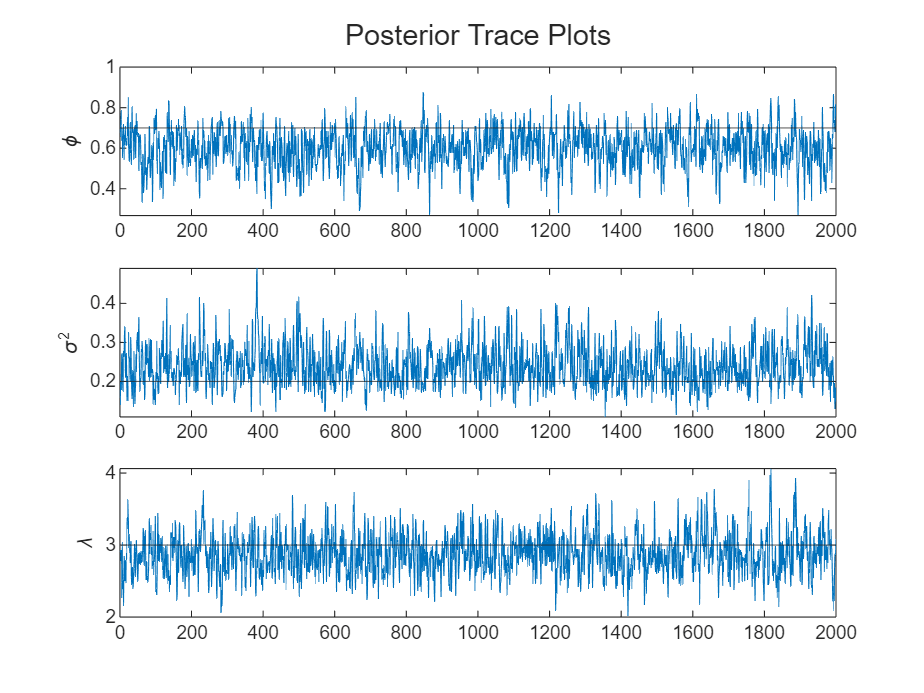
The trace plots suggest that the Markov chain settles after 100 processed draws, and significant autocorrelation among the draws exists. Therefore, you should tune the MCMC sampler.
Adjust the sampler the following ways:
Because the default burn-in period is 100 draws, specify a burn-in period of 200 (
BurnIn=200).Specify thinning the sample by keeping the first draw of each set of 10 successive draws (
Thin=10).Retain 2000 random parameter vectors (
NumDraws=2000).Set the proposal scale proportionality constant to 0.25 to increase the sample acceptance rate.
Simulate from the posterior distribution. Specify the simulated response path as observed responses, an arbitrary set of initial parameter values to initialize the MCMC algorithm, and sampler adjustments.
[ThetaPostDraws,accept] = simulate(PriorMdl,y,params,Proposal,Burnin=200,Thin=10, ...
    NumDraws=2000,Proportion=0.25);
accept
accept = 0.6860
Plot trace plots and correlograms of the parameters.
paramnames = ["\phi" "\sigma^2" "\lambda"];

figure
h = tiledlayout(numparams,1);
for j = 1:numparams
    nexttile
    plot(ThetaPostDraws(j,:))
    hold on
    yline(thetaDGP(j))
    ylabel(paramnames(j))
end
title(h,"Posterior Trace Plots")
figure
h = tiledlayout(numparams,1);
for j = 1:numparams
    nexttile
    autocorr(ThetaPostDraws(j,:));
    ylabel(paramnames(j));
    title([]);
end
title(h,"Posterior Sample Correlograms")
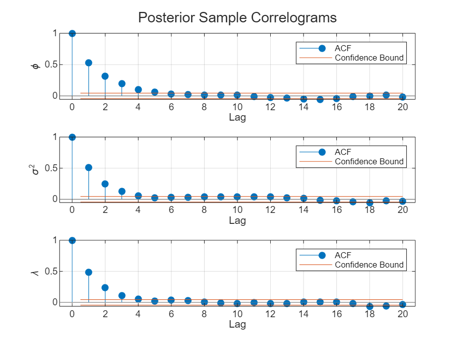
The sampler quickly settles near the true values of the parameters. The sample shows less serial correlation and little transient behavior.
Create a posterior model by setting the parameter distribution property of the prior model (ParamDistribution) to the posterior draws. Compute posterior means of each parameter.
PosteriorMdl = PriorMdl;
PosteriorMdl.ParamDistribution = ThetaPostDraws;
estParams = mean(ThetaPostDraws);
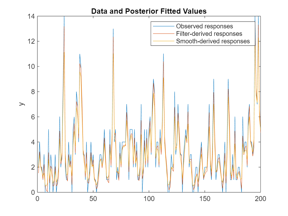
Use the posterior distribution to compute smoothed and filtered states, and then compute fitted values by transforming estimated state series to an observation series, which represents the series of Poisson means. Compare the means and the observed series.
figure
xhats = smooth(PosteriorMdl,y,estParams);
xhatf = filter(PosteriorMdl,y,estParams);
yhats = estParams(3)*exp(xhats);
yhatf = estParams(3)*exp(xhatf);
plot([y yhatf yhats])
title("Data and Posterior Fitted Values")
ylabel("y")
legend("Observed responses","Filter-derived responses", ...
    "Smooth-derived responses")
hold on
Forecast the Poisson mean into a 10-period horizon.
fh = 10;
bigN = 1000;
XF = zeros(fh + 1,bigN);
yf = zeros(fh,bigN);
XF(1,:) = xhats(end)*ones(1,bigN);
phi = PosteriorMdl.ParamDistribution(1,(end-(bigN-1)):end);
sigma2 = PosteriorMdl.ParamDistribution(2,(end-(bigN-1)):end);
lambda = PosteriorMdl.ParamDistribution(3,(end-(bigN-1)):end);
for j = 2:(fh+1)
    XF(j,:) = phi.*XF(j-1,:) + sqrt(sigma2).*randn(1,bigN);
    yf(j-1,:) = exp(XF(j,:)).*lambda;
end

yfmean = mean(yf,2);
yfci = quantile(yf,[0.025 0.975],2);
h1 = plot(T+(1:fh)',yf,Color=[0.75 0.75 0.75]);
h2 = plot(T+(1:fh)',yfmean,"k");
h3 = plot(T+(1:fh)',yfci,"r--");
axis tight
title("$h$-Day-Ahead Forecasted Volatilities",Interpreter="latex")
legend([h1(1) h2 h3(1)], ...
    ["Posterior draws" "Posterior mean" "95% credible forecast intervals"], ...
    Location="best")

Local Functions
These functions specify the state-space model parameter mappings, in distribution form, and the log prior distribution of the parameters.
function [A,B,LogY,Mean0,Cov0,StateType] = paramMap(theta)
    A = theta(1);
    B = sqrt(theta(2));
    LogY = @(y,x)y.*(x + log(theta(3)))- exp(x).*theta(3);
    Mean0 = 0;
    Cov0 = 2;
    StateType = 0;     % Stationary state process
end

function logprior = priorDistribution(theta,hyperparams)
    % Prior of phi
    m0 = hyperparams(1);
    v20 = hyperparams(2);
    pphi = makedist("normal",mu=m0,sigma=sqrt(v20));
    pphi = truncate(pphi,-1,1);
    lpphi = log(pdf(pphi,theta(1)));

    % Prior of sigma2
    a0 = hyperparams(3);
    b0 = hyperparams(4);
    lpsigma2 = -a0*log(b0) - log(gamma(a0)) + (-a0-1)*log(theta(2)) - ...
        1./(b0*theta(2));

    % Prior of lambda
    alpha0 = hyperparams(5);
    beta0 = hyperparams(6);
    plambda = makedist("gamma",alpha0,beta0);
    lplambda = log(pdf(plambda,theta(3)));

    logprior = lpphi + lpsigma2 + lplambda;
end
Consider the model in the example Draw Parameters From Posterior Distribution. Monitor the parameter draws as the MCMC sampler processes.
Create a Bayesian nonlinear state-space model (bnlssm) object that represents the DGP, and then simulate a response path.
rng(1,"twister")    % For reproducibility
T = 200;
thetaDGP = [0.7; 0.2; 3];

numparams = numel(thetaDGP);
paramnames = ["\phi" "\sigma^2" "\lambda"];

MdlXSim = arima(AR=thetaDGP(1),Variance=thetaDGP(2), ...
    Constant=0);
xsim = simulate(MdlXSim,T);
y = random("poisson",thetaDGP(3)*exp(xsim));
Create the Bayesian nonlinear state-space model template for estimation by passing function handles directly to paramMap and paramDistribution to bnlssm (the functions are in Local Functions). Tune the proposal distribution; suppress the tuning algorithm's output.
m0 = 0;
v02 = 1;
a0 = 1;
b0 = 1;
alpha0 = 3;
beta0 = 1;
hyperparams = [m0 v02 a0 b0 alpha0 beta0];

PriorMdl = bnlssm(@paramMap,@(x)priorDistribution(x,hyperparams), ...
    ObservationForm="distribution",Multipoint=["A" "LogY"]);
theta0 = [0.5; 0.1; 2];
[params,Proposal] = tune(PriorMdl,y,theta0,Display="off");
The simulate function accepts a function handle to a function accepts a structure array containing key elements of the sampler at each iteration. This function enables you to process or monitor the sampler as it runs.
Write a function that plots each parameter as simulate pulls it from the posterior distribution. This function enables you to monitor the quality of the sampler so that you can, for example, stop the process if you suspect a longer burn-in period is required, rather than wait for the sampler to complete. You can use this function only in this example.
function out = plotProgress(inputstruct,h)
    out.iter = inputstruct.Iteration;
    np = numel(h);
    for jj = np:-1:1
        out.out = inputstruct.Parameters(jj);
        addpoints(h(jj),out.iter,out.out)
        drawnow
    end
end
Simulate from the posterior distribution. Specify the simulated response path as observed responses, an arbitrary set of initial parameter values to initialize the MCMC algorithm, and adjust the sampler the following ways:
Because the default burn-in period is 100 draws, specify a burn-in period of 200 (
BurnIn=200).Specify thinning the sample by keeping the first draw of each set of 10 successive draws (
Thin=10).Retain 2000 random parameter vectors (
NumDraws=2000).Set the proposal scale proportionality constant to 0.25 to increase the sample acceptance rate.
Set up separate trace plots for the parameters. Plot the progress of the sampler by specifying a handle to the output function plotProgress.
burnin = 200;
thin = 10;
numdraws = 2000;
prop = 0.25;

figure
tiledlayout(numparams,1)
for j = numparams:-1:1
    nexttile
    h(j) = animatedline;
    hold on
    yline(thetaDGP(j),"r--")
    ylabel(paramnames(j))
end
[ThetaPostDraws,accept] = simulate(PriorMdl,y,params,Proposal,Burnin=burnin,Thin=thin, ...
    NumDraws=numdraws,Proportion=prop,OutputFunction=@(x)plotProgress(x,h));

Local Functions
These functions specify the state-space model parameter mappings, in distribution form, and the log prior distribution of the parameters.
function [A,B,LogY,Mean0,Cov0,StateType] = paramMap(theta)
    A = theta(1);
    B = sqrt(theta(2));
    LogY = @(y,x)y.*(x + log(theta(3)))- exp(x).*theta(3);
    Mean0 = 0;
    Cov0 = 2;
    StateType = 0;     % Stationary state process
end

function logprior = priorDistribution(theta,hyperparams)
    % Prior of phi
    m0 = hyperparams(1);
    v20 = hyperparams(2);
    pphi = makedist("normal",mu=m0,sigma=sqrt(v20));
    pphi = truncate(pphi,-1,1);
    lpphi = log(pdf(pphi,theta(1)));

    % Prior of sigma2
    a0 = hyperparams(3);
    b0 = hyperparams(4);
    lpsigma2 = -a0*log(b0) - log(gamma(a0)) + (-a0-1)*log(theta(2)) - ...
        1./(b0*theta(2));

    % Prior of lambda
    alpha0 = hyperparams(5);
    beta0 = hyperparams(6);
    plambda = makedist("gamma",alpha0,beta0);
    lplambda = log(pdf(plambda,theta(3)));

    logprior = lpphi + lpsigma2 + lplambda;
end
Draw posterior samples from a Bayesian nonlinear stochastic volatility model for daily S&P 500 closing returns. For a full exposition of this problem, see Fit Bayesian Stochastic Volatility Model to S&P 500 Volatility.
Consider the nonlinear state-space form of the stochastic volatility model for observed asset returns :
where:
for daily returns.
is a latent AR(1) process representing the conditional volatility series.
are are mutually independent and individually iid random standard Gaussian noise series.
The linear state-space coefficient matrices are:
The observation equation is nonlinear. Because is a standard Gaussian random variable, the conditional distribution of given and the parameters is Gaussian with a mean of 0 and standard deviation .
Load the data set Data_GlobalIdx1.mat, and then extract the S&P 500 closing prices (last column of the matrix Data).
load Data_GlobalIdx1
sp500 = Data(:,end);
T = numel(sp500);
dts = datetime(dates,ConvertFrom="datenum");
Convert the price series to returns, and then center the returns.
retsp500 = price2ret(sp500);
y = retsp500 - mean(retsp500);
retdts = dts(2:end);
The local function paramMap, which uses the distribution form for the observation equation, specifies this model structure. Unlike the parameter mapping function in Fit Bayesian Stochastic Volatility Model to S&P 500 Volatility, paramMap reduces the number of states to one for computational efficiency.
Assume a flat prior, that is, the log prior is 0 over the support of the parameters and -Inf everywhere else. The local function flatLogPrior specifies the prior.
Create a Bayesian nonlinear state-space model that specifies the model structure and prior distribution. Specify that the observation equation is in distribution form and that bnlssm functions can evaluate multiple particles simultaneously for A and LogY.
PriorMdl = bnlssm(@paramMap,@flatLogPrior,ObservationForm="distribution", ...
    Multipoint=["A" "LogY"]);
Tune the proposal distribution. Specify an arbitrarily chosen set of initial parameter values and the following settings:
Set the search interval for to (-1,1). Specified search intervals apply only to tuning the proposal.
Set the search interval for to (0,).
Specify computing the Hessian by the outer product of gradients.
For computational speed, do not sort the particles by using Hilbert sorting.
theta0 = [0.2 0 0.5];
lower = [-1; -Inf; 0];
upper = [1; Inf; Inf];
rng(1)

[params,Proposal] = tune(PriorMdl,y,theta0,Lower=lower,Upper=upper, ...
    NumParticles=500,Hessian="opg",SortParticles=false);
         Optimization and Tuning
      | Params0  Optimized  ProposalStd
----------------------------------------
 c(1) |  0.2000    0.9949      0.0030
 c(2) |   0       -0.0155      0.0116
 c(3) |  0.5000    0.1495      0.0130
Obtain a sample from the posterior distribution. Specify the optimal proposal a burn-in period of 1e4 and retain every 25th draw to reduce serial correlation among the draws. The sampler, with these settings, takes some time to complete.
burnin = 1e4;
thin = 25;

[ThetaPost,accept] = simulate(PriorMdl,y,params,Proposal, ...
    BurnIn=burnin,Thin=thin);
accept
accept = 0.5131
Determine the quality of the posterior sample by plotting trace plots of the parameter draws.
figure
plot(ThetaPost(1,:))
title("Trace Plot: \beta")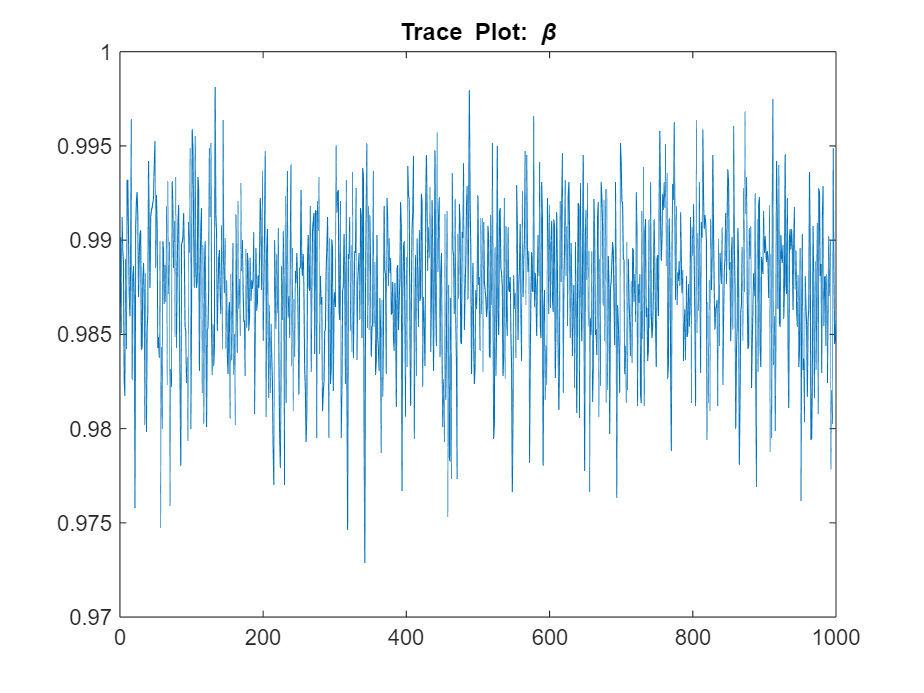
figure
plot(ThetaPost(2,:))
title("Trace Plot: \alpha")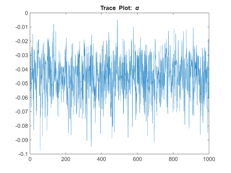
figure
plot(ThetaPost(3,:))
title("Trace Plot: \sigma")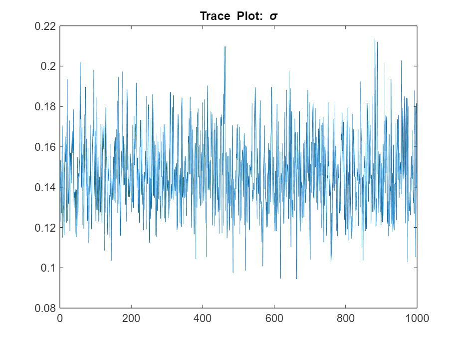
The posterior samples show good mixing with some minor serial correlation.
Local Functions
This example uses the following functions. paramMap is the parameter-to-matrix mapping function and flatLogPrior is the log prior distribution of the parameters.
function [A,B,LogY,Mean0,Cov0,StateType] = paramMap(theta)
    A = @(x) theta(2) + theta(1).*x;
    B = theta(3);
    LogY = @(y,x)-0.5.*x-0.5*365*y*y.*exp(-x);
    Mean0 = theta(2)./(1 - theta(1));
    Cov0 = (theta(3)^2)./(1 - theta(1)^2);
    StateType = 0;
end

function logprior = flatLogPrior(theta)
% flatLogPrior computes the log of the flat prior density for the three
% variables in theta. Log probabilities for parameters outside the
% parameter space are -Inf.
    paramcon = zeros(numel(theta),1);
    % theta(1) is the lag 1 term in a stationary AR(1) model. The
    % value needs to be within the unit circle.
    paramcon(1) = abs(theta(1)) >= 1 - eps;

    % alpha must be finite
    paramcon(2) = ~isfinite(theta(2));

    % Standard deviation of the state disturbance theta(3) must be positive.
    paramcon(3) = theta(3) <= eps;

    if sum(paramcon) > 0
        logprior = -Inf;
    else
        logprior = 0;   % Prior density is proportional to 1 for all values
                        % in the parameter space.
    end
end
This example compares the performance of several SMC proposal particle resampling methods for obtaining random paths of parameter values from the posterior distribution of a quasi-nonnegative constrained state space model, which models nonnegative state quantities such as interest rates and prices:
and are iid standard Gaussian random variables.
Generate Artificial Data
Consider the following data-generating process (DGP)
Generate a random series of 200 observations from the DGP.
a0 = 0.1;
a1 = 0.95;
b = 1;
d = 0.5;
theta = [a0; a1; b; d];
T = 200;

% Preallocate variables
x = zeros(T,1);
y = zeros(T,1);

rng(0,"twister") % For reproducibility
u = randn(T,1);
e = randn(T,1);

for t = 2:T
    x(t) = max(0,a0 + a1*x(t-1)) + b*u(t);
    y(t) = x(t) + d*e(t);
end
Create Bayesian Nonlinear State-Space Model
The Local Functions section contains two functions required to specify the Bayesian nonlinear state-space model: the state-space model parameter mapping function paramMap and the prior distribution of the parameters priorDistribution. You can use the functions only within this script.
The paramMap function has these qualities:
Functions can simultaneously evaluate the state equation for multiple values of
A. Therefore, you can speed up calculations by specifying theMultipoint="A"option.The observation equation is in equation form, that is, the function composing the states is nonlinear and the innovation series is additive, linear, and Gaussian.
The priorDistribution function specifies a flat prior, which has a density that is proportional to 1 everywhere in the parameter space; it constrains the error standard deviations to be positive.
Create a Bayesian nonlinear state-space model characterized by the system.
PriorMdl = bnlssm(@paramMap,@priorDistribution,Multipoint="A");Draw Random Parameter Paths from Posterior Using Each Proposal Sampler Method
Obtain random parameter paths from the joint posterior distribution using the bootstrap, optimal, and one-pass unscented particle resampling methods. Tune the sampler initialized from a randomly drawn set of values in [0,1], thin the sample by a factor of 10, specify a burn-in period of 100, and draw 1000 paths.
numDraws = 1000;
smcMethod = ["bootstrap" "optimal" "unscented"];
for j = 3:-1:1 % Set last element first to preallocate entire cell vector
    params0 = rand(4,1);
    [params,Proposal] = tune(PriorMdl,y,params0,Display="off",NewSamples=smcMethod(j));
    thetaSim{j} = simulate(PriorMdl,y,params,Proposal,NewSamples=smcMethod(j), ...
        NumDraws=numDraws,Thin=10,Burnin=100);
end
Separately for each parameter, draw histograms of the posterior draws for each method on the same plot.
figure
tiledlayout(2,2)
varnames = ["a0" "a1" "b" "d"];
for j = 1:numel(theta)
    nexttile
    h1 = histogram(thetaSim{1}(j,:));
    hold on
    h2 = histogram(thetaSim{2}(j,:));
    h3 = histogram(thetaSim{3}(j,:));
    h4 = xline(theta(j),"--",LineWidth=2);
    hold off
    title(varnames(j))
end
legend([h1 h2 h3 h4],[smcMethod "True"])
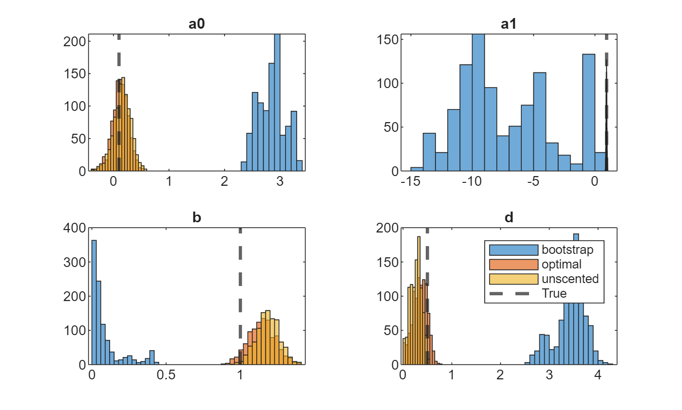
In this case, the optimal and one-pass unscented methods yield distributions closer to the true values than the bootstrap method.
Local Functions
These functions specify the state-space model parameter mappings, in equation form, and log prior distribution of the parameters.
function [A,B,C,D,mean0,Cov0] = paramMap(params)
    a0 = params(1);
    a1 = params(2);
    b = params(3);
    d = params(4);
    A = @(x) max(0,a0+a1.*x);
    B = b;
    C = 1;
    D = d;
    mean0 = 0;
    Cov0 = 1;
end

function logprior = priorDistribution(theta)
    paramconstraints = theta(3:4) <= 0; % b and d are greater than 0
    if(sum(paramconstraints))
        logprior = -Inf;
    else
        logprior = 0;   % Prior density is proportional to 1 for all values
                        % in the parameter space.
    end
end
Input Arguments
Observed response data, specified as a numeric matrix or a cell vector of numeric vectors.
If
PriorMdlis time invariant with respect to the observation equation,Yis a T-by-n matrix. Each row of the matrix corresponds to a period and each column corresponds to a particular observation in the model. T is the sample size and n is the number of observations per period. The last row ofYcontains the latest observations.If
PriorMdlis time varying with respect to the observation equation,Yis a T-by-1 cell vector.Y{t}contains an nt-dimensional vector of observations for period t, where t = 1, ..., T. For linear observation models, the corresponding dimensions of the coefficient matrices, outputs ofPriorMdl.ParamMap,C{t}, andD{t}must be consistent with the matrix inY{t}for all periods. For nonlinear observation models, the dimensions of the inputs and outputs associated with the observations must be consistent. Regardless of model type, the last cell ofYcontains the latest observations.
NaN elements indicate missing observations. For details on how
simulate accommodates missing observations, see Algorithms.
Data Types: double | cell
Initial parameter values for the parameters Θ, specified as a
numParams-by-1 numeric vector. Elements of
params0 must correspond to the elements of the first input
arguments of PriorMdl.ParamMap and
PriorMdl.ParamDistribution.
Data Types: double
MH sampler proposal distribution covariance/scale matrix for the parameters Θ, up to
the proportionality constant Proportion, specified as a
numParams-by-numParams, positive-definite
numeric matrix. Elements of Proposal must correspond to elements in
params0.
The proposal distribution is multivariate normal or Student's t
with DoF degrees of freedom (for details, see
DoF).
Data Types: double
Name-Value Arguments
Specify optional pairs of arguments as
Name1=Value1,...,NameN=ValueN, where Name is
the argument name and Value is the corresponding value.
Name-value arguments must appear after other arguments, but the order of the
pairs does not matter.
Example: simulate(PriorMdl,Y,params0,Proposal,NumDraws=1e3,Thin=4,DoF=10)
uses the multivariate t10 distribution for the MH
proposal, draws 4e3 random vectors of parameters, and thins the sample to
reduce serial correlation by discarding every 3 draws until it retains
1e3 draws.
Number of MCMC sampler draws from the posterior distribution Π(θ|Y), specified as a positive integer.
Example: NumDraws=1e5
Data Types: double
Number of draws to remove from the beginning of the sample to reduce transient effects,
specified as a nonnegative scalar. For details on how simulate
reduces the full sample, see Algorithms.
Tip
To help you specify the appropriate burn-in period size:
Determine the extent of the transient behavior in the sample by setting the
BurnInname-value argument to0.Simulate a few thousand observations by using
simulate.Create trace plots.
Example: BurnIn=1000
Data Types: double
Adjusted sample size multiplier, specified as a positive integer.
The actual sample size is BurnIn +
NumDraws*Thin. After discarding the burn-in,
simulate discards every Thin –
1 draws, and then retains the next draw. For more details on how
simulate reduces the full sample, see Algorithms.
Tip
To reduce potential large serial correlation in the posterior sample, or to reduce the memory
consumption of the output sample, specify a large
value for Thin.
Example: Thin=5
Data Types: double
Proposal distribution degrees of freedom for parameter updates using the MH sampler, specified as a value in this table.
| Value | MH Proposal Distribution |
|---|---|
| Positive scalar | Multivariate t with DoF degrees of freedom |
Inf | Multivariate normal |
The following options specify other aspects of the proposal distribution:
Proportion— Optional proportionality constant that scalesProposalCenter— Optional expected value
Example: DoF=10
Data Types: double
Proposal scale matrix proportionality constant, specified as a positive scalar.
Tip
For higher proposal acceptance rates, experiment with relatively small values for Proportion.
Example: Proportion=1
Data Types: double
Proposal distribution center, specified as a value in this table.
| Value | Description |
|---|---|
numParams-by-1 numeric vector | simulate uses the independence Metropolis-Hastings sampler. Center is the center of the proposal distribution. |
[] (empty array) | simulate uses the random-walk Metropolis-Hastings sampler. The center of the proposal density is the current state of the Markov chain. |
Example: Center=ones(10,1)
Data Types: double
Number of particles for SMC, specified as a positive integer.
Example: NumParticles=1e4
Data Types: double
Since R2025a
SMC proposal (importance) distribution, specified as a value in this table.
| Value | SMC Sampler | Description |
|---|---|---|
| Auxiliary filter [11] | SMC samples particles by using a reweight-resample strategy, which uses local approximations of the nonlinear state-space model and is informed by the observations. This option is
available only for models with observation noise (nonzero
|
"bootstrap" | Bootstrap forward filter [7] | SMC samples particles form the state transition distribution (observations do not inform the sampler). This option
is available only for models with observation noise (nonzero
This method has a relatively low computational cost, but it does not inform the routine of the current observations, which can increase the Monte Carlo sampling variance. |
"optimal" | Conditionally optimal proposal [4] | SMC samples particles from the one-step filtering distribution with incremental weights proportional to the likelihood (observations inform the sampler). The weights have minimum variance. This option is available for the following tractable models supplied in equation form:
|
"unscented" | Unscented transformation [12] | SMC proposal distribution is the one-step filtering distribution approximated by the unscented transformation (observations inform the sampler). This option is
available only for models in equation form with observation noise
(nonzero By default, this option
uses the filtered state mean as the representative point, around
which the algorithm generates sigma points. To specify all particles
as representative points for the unscented transformation, set
|
Example: NewSamples="unscented"
Data Types: char | string
Since R2025a
Flag to apply unscented transformation to all particles, specified as a value in this table.
| Value | Description |
|---|---|
false | The filtered state mean is the representative point, around which the algorithm generates sigma points. This
option is less computationally expensive than
|
true | All particles are the representative points. This option is more computationally expensive than the default, but it can yield a higher-quality proposal distribution. |
Example: MultiPassUnscented=false
Data Types: logical
SMC resampling method, specified as a value in this table.
| Value | Description |
|---|---|
"multinomial" | At time t, the set of previously generated particles (parent set) follows a standard multinomial distribution, with probabilities proportional to their weights. An offspring set is resampled with replacement from the parent set [1]. |
"residual" | Residual sampling, a modified version of multinomial resampling that can produce an estimator with lower variance than the multinomial resampling method [8]. |
"systematic" | Systematic sampling, which produces an estimator with lower variance than the multinomial resampling method [3]. |
Resampling methods downsample insignificant particles to achieve a smaller estimator variance than if no resampling is performed and to avoid sampling from a degenerate proposal [5].
Example: Resample="residual"
Data Types: char | string
Effective sample size threshold, below which simulate resamples particles, specified as a nonnegative scalar. For more details, see [5], Ch. 12.3.3.
Tip
To resample during every period, set
Cutoff=numparticles, wherenumparticlesis the value of theNumParticlesname-value argument.To avoid resampling, set
Cutoff=0.
Example: Cutoff=0.75*numparticles
Data Types: double
Flag for sorting particles before resampling, specified as a value in this table.
| Value | Description |
|---|---|
true | simulate sorts the generated particles before resampling them. |
false | simulate does not sort the generated particles. |
When SortParticles=true, simulate uses Hilbert
sorting during the SMC routine to sort the particles. This action can reduce Monte Carlo
variation, which is useful when you compare loglikelihoods resulting from evaluating several
params arguments that are close to each other [3]. However, the sorting routine
requires more computation resources, and can slow down computations, particularly in
problems with a high-dimensional state variable.
Example: SortParticles=false
Data Types: logical
Custom function of particles and normalized weights for monitoring the SMC, specified as a function handle (@customstats).
The associated function signature must have this form:
function stat = customStatistics(particles,weights)
where:
customStatisticsparticlesis the mt-by-NumParticleschosen particles at forward-filtering time t of the SMC routine.weightsis the 1-by-NumParticlesnormalized importance weights, corresponding toparticles, at forward-filtering time t of the SMC routine.statis the evaluation ofcustomStatisticsatparticlesandweightsat forward-filtering time t of the SMC routine. For example,statcan be a numeric vector or structure array.
Example: You can return the particles and weights at each filtering step by setting CustomStatistics=@customstats, where you write customstats to return those inputs in a structure array: stat.p = particles; stat.w = weights;
Data Types: function_handle
Autocorrelation of normal random numbers for particle generation and resampling during SMC, specified as a positive scalar in the interval [0,1].
For
0,simulaterandomly generates new numbers independently of those previously drawn.For
1,simulategenerates an initial set of random numbers, but uses those same numbers for the duration of SMC sampling.For a value between 0 and 1, exclusive,
simulategenerates the random numbers of sample j, sj, using , where zj is a set of iid standard normal variates.
Example: Autocorrelation=0.5
Data Types: double
Function that simulate calls after each MCMC iteration,
specified as a function handle. simulate saves the outputs of
the specified function after each iteration and returns them in the
Output output argument. You write the function, which can
perform arbitrary calculations, such as computing or plotting custom statistics at
each iteration.
Suppose outputfcnoutputfcn
function Output = outputfcn(Input)
	...
end
simulate passes
Input| Field | Description | Value |
|---|---|---|
Iteration | Current iteration | Numeric scalar |
Parameters | Current values of the parameters θ | Numeric vector |
LogPosteriorDensity | Log posterior density evaluated at current parameters and conditioned on latent variables | Numeric scalar |
RND | Information describing normal random variables used by the filter
routine (see filter) | Structure array |
Particles | Current (weighted) particles for approximating the filtering distribution (final state distribution). | 1-by-NumParticles numeric vector |
Weights | Current particle weights | 1-by-T numeric vector |
FinalStates | Random draw from the weighted particles, as a posterior sample of the final states | mT-by-1 numeric vector |
FilteredStates | Current estimate of the mean of the filtered states; an estimate of | mt-by-1 numeric vector |
FilteredStatesCov | Current estimate of the variance-covariance matrix of the filtered states; an estimate of | mt-by-mt numeric matrix |
Mdl | Input model PrioirMdl | bnlssm
object |
Y | Observations | The value of the input Y |
PreviousOutput | Output of the previous iteration | Structure array with fields in this table |
OutputoutputfcnOutputsimulate
concatenates the outputs of all iterations and returns a
k-by-NumDraws matrix of the same type. If
simulate cannot horizontally concatenate the outputs of all
iterations, simulate returns a
1-by-NumDraws cell array instead, where successive cells contain
the output of corresponding iterations.
Example: OutputFunction=@outputfcn
Data Types: function_handle
Output Arguments
Proposal acceptance rate, returned as a positive scalar in [0,1].
Custom function OutputFunction output concatenated over all MCMC iterations, returned as a matrix or cell vector. Output has NumDraws columns, and the number of rows depends on the size of the output at each iteration. The data type of the entries of Output depends on the operations of the output function.
Tips
In general, you can reproduce results by setting
rng. However, to pass normal random numbers generated byfilteras particles tosimulate, set theRNDargument to those random numbers.Unless you set
Cutoff=0,simulateresamples particles according to the specified resampling methodResample. Although resampling particles with high weights improves the results of the SMC, you should also allow the sampler traverse the proposal distribution to obtain novel, high-weight particles. To do this, experiment withCutoff.Acceptance rates from
acceptthat are relatively close to 0 or 1 indicate that the Markov chain does not sufficiently explore the posterior distribution. To obtain an appropriate acceptance rate for your data, tune the sampler by implementing one of the following procedures.Use the
tunefunction to search for the posterior mode by numerical optimization.tunereturns optimized parameters and the proposal scale matrix, which is proportional to the negative Hessian matrix evaluated at the posterior mode. Pass the optimized parameters and the proposal scale tosimulate, and tune the proportionality constant by using theProportionname-value argument. Small values ofProportiontend to increase the proposal acceptance rates of the MH sampler.Perform a multistage simulation:
Choose an initial value for the input
Proposaland simulate draws from the posterior.Compute the sample covariance matrix, and pass the result to
simulateas an updated value forProposal.Repeat steps 1 and 2 until
acceptis reasonable for your data.
Avoid an arbitrary choice of the initial state distribution.
bnlssmfunctions generate the initial particles from the specified initial state distribution, which impacts the performance of the nonlinear filter. If the initial state specification is bad enough, importance weights concentrate on a small number of particles in the first SMC iteration, which might produce unreasonable filtering results. This vulnerability of the nonlinear model behavior contrasts with the stability of the Kalman filter for the linear model, in which the initial state distribution usually has little impact on the filter because the prior is washed out as it processes data.
Algorithms
simulateaccommodates missing data by not updating filtered state estimates corresponding to missing observations. In other words, suppose there is a missing observation at period t. Then, the state forecast for period t based on the previous t – 1 observations and filtered state for period t are equivalent.
References
[1] Andrieu, Christophe, Arnaud Doucet, and Roman Holenstein. "Particle Markov Chain Monte Carlo Methods." Journal of the Royal Statistical Society Series B: Statistical Methodology 72 (June 2010): 269–342. https://doi.org/10.1111/j.1467-9868.2009.00736.x.
[2] Andrieu, Christophe, and Gareth O. Roberts. "The Pseudo-Marginal Approach for Efficient Monte Carlo Computations." Ann. Statist. 37 (April 2009): 697–725. https://dx.doi.org/10.1214/07-AOS574.
[3] Deligiannidis, George, Arnaud Doucet, and Michael Pitt. "The Correlated Pseudo-Marginal Method." Journal of the Royal Statistical Society, Series B: Statistical Methodology 80 (June 2018): 839–870. https://doi.org/10.1111/rssb.12280.
[4] Doucet, Arnaud, Simon Godsill, and Christophe Andrieu. "On Sequential Monte Carlo Sampling Methods for Bayesian Filtering." Statistics and Computing 10 (July 2000): 197–208. https://doi.org/10.1023/A:1008935410038.
[5] Durbin, J, and Siem Jan Koopman. Time Series Analysis by State Space Methods. 2nd ed. Oxford: Oxford University Press, 2012.
[6] Fernández-Villaverde, Jesús, and Juan F. Rubio-Ramírez. "Estimating Macroeconomic Models: A Likelihood Approach." Review of Economic Studies 70(October 2007): 1059–1087. https://doi.org/10.1111/j.1467-937X.2007.00437.x.
[7] Gordon, Neil J., David J. Salmond, and Adrian F. M. Smith. "Novel Approach to Nonlinear/Non-Gaussian Bayesian State Estimation." IEE Proceedings F Radar and Signal Processing 140 (April 1993): 107–113. https://doi.org/10.1049/ip-f-2.1993.0015.
[8] Liu, Jun, and Rong Chen. "Sequential Monte Carlo Methods for Dynamic Systems." Journal of the American Statistical Association 93 (September 1998): 1032–1044. https://dx.doi.org/10.1080/01621459.1998.10473765.
[9] Hastings, Wilfred K. "Monte Carlo Sampling Methods Using Markov Chains and Their Applications." Biometrika 57 (April 1970): 97–109. https://doi.org/10.1093/biomet/57.1.97.
[10] Metropolis, Nicholas, Rosenbluth, Arianna. W., Rosenbluth, Marshall. N., Teller, Augusta. H., and Teller, Edward. "Equation of State Calculations by Fast Computing Machines." The Journal of Chemical Physics 21 (June 1953): 1087–92. https://doi.org/10.1063/1.1699114.
[11] Pitt, Michael K., and Neil Shephard. "Filtering via Simulation: Auxiliary Particle Filters." Journal of the American Statistical Association 94 (June 1999): 590–599. https://doi.org/10.1080/01621459.1999.10474153.
[12] van der Merwe, Rudolph, Arnaud Doucet, Nando de Freitas, and Eric Wan. "The Unscented Particle Filter." Advances in Neural Information Processing Systems 13 (November 2000). https://dl.acm.org/doi/10.5555/3008751.3008833.
Version History
Introduced in R2024bIn addition to the supported SMC particle resampling methods, you can set the NewSamples name-value argument to "auxiliary" to specify the auxiliary particle filter. The auxiliary particle filter resembles the conditionally optimal proposal method ("optimal"), but its reweight-resample strategy uses local approximations of the smoothing distribution of the target, rather than requiring a closed form. Therefore, unlike the conditionally optimal proposal method, it supports both equation-form and distribution-form models.
While the SMC routine implements forward filtering, it resamples particles to align them to
the target distribution. The NewSamples name-value argument enables you
to choose how the SMC sampler chooses the particles. The supported algorithms are the
bootstrap forward filter ("bootstrap"), the conditionally optimal
proposal ("optimal"), and the unscented transformation
("unscented).
By default, the unscented transformation uses the filtered state mean as the representative
point, around which sigma points are generated. The MultiPassUnscented
name-value argument enables you to specify all particles as representative points for the
unscented transformation.
Before R2025a, the functions implement forward filtering using only the bootstrap filter.
See Also
Objects
Functions
MATLAB Command
You clicked a link that corresponds to this MATLAB command:
Run the command by entering it in the MATLAB Command Window. Web browsers do not support MATLAB commands.
Select a Web Site
Choose a web site to get translated content where available and see local events and offers. Based on your location, we recommend that you select: .
You can also select a web site from the following list
How to Get Best Site Performance
Select the China site (in Chinese or English) for best site performance. Other MathWorks country sites are not optimized for visits from your location.
Americas
- América Latina (Español)
- Canada (English)
- United States (English)
Europe
- Belgium (English)
- Denmark (English)
- Deutschland (Deutsch)
- España (Español)
- Finland (English)
- France (Français)
- Ireland (English)
- Italia (Italiano)
- Luxembourg (English)
- Netherlands (English)
- Norway (English)
- Österreich (Deutsch)
- Portugal (English)
- Sweden (English)
- Switzerland
- United Kingdom (English)