Main Content

armairf

Generate or plot ARMA model impulse responses

Description

The armairf function returns or plots the impulse response functions (IRFs) of the variables in a univariate or vector (multivariate) autoregressive moving average (ARMA) model specified by arrays of coefficients or lag operator polynomials.

Alternatively, you can return an IRF from a fully specified (for example, estimated) model object by using the function in this table.

IRFs trace the effects of an innovation shock to one variable on the response of all variables in the system. In contrast, the forecast error variance decomposition (FEVD) provides information about the relative importance of each innovation in affecting all variables in the system. To estimate FEVDs of univariate or multivariate ARMA models, see armafevd.

example

armairf(ar0,ma0) plots, in separate figures, the impulse response function of the numVars time series variables that compose an ARMA(p,q) model. The autoregressive (AR) and moving average (MA) coefficients of the model are ar0 and ma0, respectively. Each figure contains numVars line plots representing the responses of a variable from applying a one-standard-deviation shock, at time 0, to all variables in the system over the forecast horizon.

The armairf function:

  • Accepts vectors or cell vectors of matrices in difference-equation notation

  • Accepts LagOp lag operator polynomials corresponding to the AR and MA polynomials in lag operator notation

  • Accommodates time series models that are univariate or multivariate, stationary or integrated, structural or in reduced form, and invertible or noninvertible

  • Assumes that the model constant c is 0

example

armairf(ar0,ma0,Name=Value) plots the numVars IRFs with additional options specified by one or more name-value arguments. For example, NumObs=10,Method="generalized" specifies a 10-period forecast horizon and the estimation of the generalized IRF.

example

Y = armairf(___) returns the numVars IRFs using any of the input argument combinations in the previous syntaxes.

armairf(ax,___) plots to the axes specified in ax instead of the axes in new figures. The option ax can precede any of the input argument combinations in the previous syntaxes.

[Y,h] = armairf(___) additionally returns handles to plotted graphics objects. Use elements of h to modify properties of the returned plots.

Examples

collapse all

Plot the entire IRF of the univariate ARMA(2,1) model

yt=0.3yt-1-0.1yt-2+εt+0.05εt-1.

Create vectors for the autoregressive and moving average coefficients as you encounter them in the model as expressed in difference-equation notation.

AR0 = [0.3 -0.1];
MA0 = 0.05;

Plot the orthogonalized IRF of yt.

armairf(AR0,MA0);

Figure contains an axes object. The axes object with title Orthogonalized IRF of Variable 1, xlabel Observation Time, ylabel Response contains an object of type line.

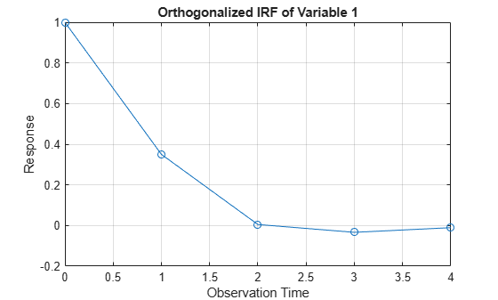
The impulse response fades after four periods.

Alternatively, create an ARMA model that represents yt. Specify 1 for the variance of the innovations, and no model constant.

Mdl = arima(AR=AR0,MA=MA0,Variance=1,Constant=0);

Mdl is an arima model object.

Plot the IRF using Mdl.

impulse(Mdl);

Figure contains an axes object. The axes object with title Impulse Response, xlabel Observation Time, ylabel Response contains an object of type stem.

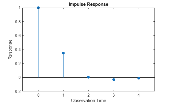
impulse uses a stem plot, whereas armairf uses a line plot. However, the IRFs in the two implementations are equal because the variance of the ARMA model is 1.

Plot the entire generalized IRF of the univariate ARMA(2,1) model

(1-0.3L+0.1L2)yt=(1+0.05L)εt.

Because the model is in lag operator form, create the polynomials using the coefficients as you encounter them in the model.

AR0Lag = LagOp([1 -0.3 0.1])
AR0Lag = 
    1-D Lag Operator Polynomial:
    -----------------------------
        Coefficients: [1 -0.3 0.1]
                Lags: [0 1 2]
              Degree: 2
           Dimension: 1
MA0Lag = LagOp([1 0.05])
MA0Lag = 
    1-D Lag Operator Polynomial:
    -----------------------------
        Coefficients: [1 0.05]
                Lags: [0 1]
              Degree: 1
           Dimension: 1

AR0Lag and MA0Lag are LagOp lag operator polynomials representing the autoregressive and moving average lag operator polynomials, respectively.

Plot the generalized IRF by passing in the lag operator polynomials.

armairf(AR0Lag,MA0Lag,Method="generalized");

Figure contains an axes object. The axes object with title Generalized IRF of Variable 1, xlabel Observation Time, ylabel Response contains an object of type line.

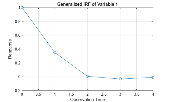
The IRF is equivalent to the IRF in Plot Orthogonalized IRF of Univariate ARMA Model.

Plot the entire IRF of the structural vector autoregression moving average model (VARMA(8,4))

{[10.2-0.10.031-0.150.9-0.251]-[-0.50.20.10.30.1-0.1-0.40.20.05]L4-[-0.050.020.010.10.010.001-0.040.020.005]L8}yt={[100010001]+[-0.020.030.30.0030.0010.010.30.010.01]L4}εt

where yt=[y1ty2ty3t] and εt=[ε1tε2tε3t].

The VARMA model is in lag operator notation because the response and innovation vectors are on opposite sides of the equation.

Create a cell vector containing the VAR matrix coefficients. Because this model is a structural model in lag operator notation, start with the coefficient of yt and enter the rest in order by lag. Construct a vector that indicates the degree of the lag term for the corresponding coefficients (the structural-coefficient lag is 0).

var0 = {[1 0.2 -0.1; 0.03 1 -0.15; 0.9 -0.25 1],...
    -[-0.5 0.2 0.1; 0.3 0.1 -0.1; -0.4 0.2 0.05],...
    -[-0.05 0.02 0.01; 0.1 0.01 0.001; -0.04 0.02 0.005]};
var0Lags = [0 4 8];

Create a cell vector containing the VMA matrix coefficients. Because this model is in lag operator notation, start with the coefficient of εt and enter the rest in order by lag. Construct a vector that indicates the degree of the lag term for the corresponding coefficients.

vma0 = {eye(3),...
    [-0.02 0.03 0.3; 0.003 0.001 0.01; 0.3 0.01 0.01]};
vma0Lags = [0 4];

Construct separate lag operator polynomials that describe the VAR and VMA components of the VARMA model.

VARLag = LagOp(var0,Lags=var0Lags);
VMALag = LagOp(vma0,Lags=vma0Lags);

Plot the generalized IRF of the VARMA model.

figure;
armairf(VARLag,VMALag,Method="generalized");

Figure contains an axes object. The axes object with title Generalized IRF of Variable 1, xlabel Observation Time, ylabel Response contains 3 objects of type line. These objects represent Shock to variable 1, Shock to variable 2, Shock to variable 3.

Figure contains an axes object. The axes object with title Generalized IRF of Variable 2, xlabel Observation Time, ylabel Response contains 3 objects of type line. These objects represent Shock to variable 1, Shock to variable 2, Shock to variable 3.

Figure contains an axes object. The axes object with title Generalized IRF of Variable 3, xlabel Observation Time, ylabel Response contains 3 objects of type line. These objects represent Shock to variable 1, Shock to variable 2, Shock to variable 3.

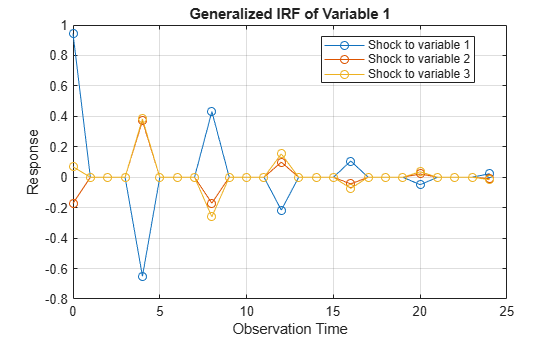
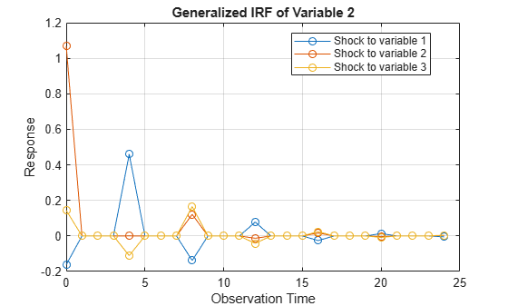
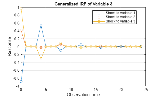
armairf returns three figures. Figure k contains the generalized IRF of variable k to a shock applied to all other variables at time 0. Because all IRFs fade after a finite number of periods, the VARMA model is stable.

Compute the entire orthogonalized IRF of the univariate ARMA(2,1) model

yt=0.3yt-1-0.1yt-2+εt+0.05εt-1.

Create vectors for the autoregressive and moving average coefficients as you encounter them in the model, which is expressed in difference-equation notation.

AR0 = [0.3 -0.1];
MA0 = 0.05;

Plot the orthogonalized IRF of yt.

y = armairf(AR0,MA0)
y = 5×1

    1.0000
    0.3500
    0.0050
   -0.0335
   -0.0105

y is a 5-by-1 vector of impulse responses. y(1) is the impulse response for time t=0, y(2) is the impulse response for time t=1, and so on. The IRF fades after period t=4.

Alternatively, create an ARMA model that represents yt. Specify 1 for the variance of the innovations, and no model constant.

Mdl = arima(AR=AR0,MA=MA0,Variance=1,Constant=0);

Mdl is an arima model object.

Plot the IRF of the ARIMA model Mdl.

y = impulse(Mdl)
y = 5×1

    1.0000
    0.3500
    0.0050
   -0.0335
   -0.0105

The IRFs in the two implementations are equivalent.

Compute the generalized IRF of the 2-D VAR(3) model

yt=[1-0.2-0.10.3]yt-1-[0.75-0.1-0.050.15]yt-2+[0.55-0.02-0.010.03]yt-3+εt.

In the equation, yt=[y1,ty2,t], εt=[ε1,tε2,t], and, for all t, εt is Gaussian with mean zero and covariance matrix

Σ=[0.5-0.1-0.10.25].

Create a cell vector of matrices for the autoregressive coefficients as you encounter them in the model as expressed in difference-equation notation. Specify the innovation covariance matrix.

AR1 = [1 -0.2; -0.1 0.3];
AR2 = -[0.75 -0.1; -0.05 0.15];
AR3 = [0.55 -0.02; -0.01 0.03];
ar0 = {AR1 AR2 AR3};

InnovCov = [0.5 -0.1; -0.1 0.25];

Compute the entire generalized IRF of yt. Because no MA terms exist, specify an empty array ([]) for the second input argument.

Y = armairf(ar0,[],Method="generalized",InnovCov=InnovCov);
size(Y)
ans = 1×3

    31     2     2

Y(10,1,2)
ans = -0.0116

Y is a 31-by-2-by-2 array of impulse responses. Rows correspond to times 0 through 30 in the forecast horizon, columns correspond to the variables that armairf shocks at time 0, and pages correspond to the impulse response of the variables in the system. For example, the generalized impulse response of variable 2 at time 10 in the forecast horizon, when variable 1 is shocked at time 0, is Y(11,1,2) = -0.0116.

armairf satisfies the stopping criterion after 31 periods. You can specify to stop sooner using the NumObs name-value argument. This practice is beneficial when the system has many variables.

Compute and display the generalized impulse responses for the first 10 periods.

Y10 = armairf(ar0,[],Method="generalized",InnovCov=InnovCov, ...
    NumObs=10)
Y10 = 
Y10(:,:,1) =

    0.7071   -0.2000
    0.7354   -0.3000
    0.2135   -0.1340
    0.0526   -0.0112
    0.2929   -0.0772
    0.3717   -0.1435
    0.1872   -0.0936
    0.0730   -0.0301
    0.1360   -0.0388
    0.1841   -0.0674


Y10(:,:,2) =

   -0.1414    0.5000
   -0.1131    0.1700
   -0.0509   -0.0040
    0.0058   -0.0113
    0.0040   -0.0003
   -0.0300    0.0100
   -0.0325    0.0133
   -0.0082    0.0054
   -0.0001   -0.0003
   -0.0116    0.0028

Y10 is a 10-by-2-by-2 array of impulse responses. Rows correspond to times 0 through 9 in the forecast horizon.

The impulse responses appear to fade with increasing time, which suggests a stable system.

Copyright 2018 The MathWorks, Inc.

Input Arguments

collapse all

Autoregressive coefficients of the ARMA(p,q) model, specified as a numeric vector, cell vector of square numeric matrices, or LagOp lag operator polynomial object. If ar0 is a vector (numeric or cell), then the coefficient of yt is the identity (eye(numVars)).

For an MA model, specify an empty array or cell ([] or {}).

  • For univariate time series models, ar0 is a numeric vector, cell vector of scalars, or one-dimensional LagOp lag operator polynomial. For vectors, ar0 has length p, and the elements correspond to lagged responses that compose the AR polynomial in difference-equation notation. In other words, ar0(j) or ar0{j} is the coefficient of yt-j, j = 1,…,p.

  • For numVars-dimensional time series models, ar0 is a cell vector of numVars-by-numVars numeric matrices or a numVars-dimensional LagOp lag operator polynomial. For cell vectors:

    • ar0 has length p.

    • ar0 and ma0 each must contain numVars-by-numVars matrices. For each matrix, row k and column k correspond to variable k in the system k = 1,…,numVars.

    • The elements of ar0 correspond to the lagged responses that compose the AR polynomial in difference equation notation. In other words, ar0{j} is the coefficient matrix of vector yt-j, j = 1,…,p. For all AR coefficient matrices, row k contains the AR coefficients in the equation of the variable ykt, and column k contains the coefficients of variable ykt within the equations. The row and column order of all autoregressive and moving average coefficients must be consistent.

  • For LagOp lag operator polynomials:

    • Coefficients in the Coefficients property correspond to the lags of yt in the Lags property.

    • Specify a model in reduced form by supplying the identity for the first coefficient (eye(numVars)).

    • armairf composes the model using lag operator notation. In other words, when you work from a model in difference-equation notation, negate the AR coefficients of the lagged responses to construct the lag operator polynomial equivalent.

For example, consider yt=0.5yt10.8yt2+εt0.6εt1+0.08εt2. The model is in difference-equation form. To compute the impulse responses, enter the following in the command line.

ar0 = [0.5 -0.8];
ma0 = [-0.6 0.08];
y = armairf(ar0,ma0);

The ARMA model written in lag-operator notation is (10.5L+0.8L2)yt=(10.6L+0.08L2)εt. The AR coefficients of the lagged responses are negated compared to the corresponding coefficients in difference-equation format. To obtain the same result using lag operator notation, enter the following in the command line.

ar0 = LagOp({1 -0.5 0.8});
ma0 = LagOp({1 -0.6 0.08});
y = armairf(ar0, ma0);

Moving average coefficients of the ARMA(p,q) model, specified as a numeric vector, cell vector of square numeric matrices, or LagOp lag operator polynomial object. If ma0 is a vector (numeric or cell), then the coefficient of εt is the identity (eye(numVars)).

For an AR model, specify an empty array or cell ([] or {}).

  • For univariate time series models, ma0 is a numeric vector, cell vector of scalars, or one-dimensional LagOp lag operator polynomial. For vectors, ma0 has length q, and the elements correspond to lagged innovations that compose the AR polynomial in difference-equation notation. In other words, ma0(j) or ma0{j} is the coefficient of εt-j, j = 1,…,q.

  • For numVars-dimensional time series models, ma0 is a cell vector of numeric numVars-by-numVars numeric matrices or a numVars-dimensional LagOp lag operator polynomial. For cell vectors:

    • ma0 has length q.

    • ar0 and ma0 each must contain numVars-by-numVars matrices. For each matrix, row k and column k correspond to variable k in the system k = 1,…,numVars.

    • The elements of ma0 correspond to the lagged responses that compose the MA polynomial in difference-equation notation. In other words, ma0{j} is the coefficient matrix of εt-j, j = 1,…,q. For all MA coefficient matrices, row k contains the MA coefficients in the equation of the variable εkt, and column k contains the coefficients of εkt within the equations. The row and column order of all autoregressive and moving average coefficient matrices must be consistent.

  • For LagOp lag operator polynomials, coefficients in the Coefficients property correspond to the lags of εt in the Lags property.

    To specify a model in reduced form, supply the identity (eye(numVars)) for the coefficient that corresponds to lag 0.

Axes on which to plot the IRF of each variable, specified as a vector of Axes objects with length equal to numVars.

By default, armairf plots impulse responses on axes in separate figures.

Name-Value Arguments

Specify optional pairs of arguments as Name1=Value1,...,NameN=ValueN, where Name is the argument name and Value is the corresponding value. Name-value arguments must appear after other arguments, but the order of the pairs does not matter.

Before R2021a, use commas to separate each name and value, and enclose Name in quotes.

Example: Method="generalized",NumObs=10 specifies to compute the generalized IRF for 10 periods.

Covariance matrix of the ARMA(p,q) model innovations εt, specified as a numeric scalar or a numVars-by-numVars numeric matrix. InnovCov must be a positive scalar or a positive definite matrix.

The default value is eye(numVars).

Example: InnovCov=0.2

Data Types: double

Forecast horizon, or the number of periods for which armairf computes the IRF, specified as a positive integer. NumObs specifies the number of observations to include in the IRF (the number of rows in Y).

By default, armairf determines NumObs by the stopping criteria of mldivide.

Example: NumObs=10

Data Types: double

IRF computation method, specified as a value in this table.

ValueDescription
"orthogonalized"Compute impulse responses using orthogonalized, one-standard-deviation innovation shocks. armairf uses the Cholesky factorization of InnovCov for orthogonalization.
"generalized"Compute impulse responses using one-standard-deviation innovation shocks.

Example: 'Method',"generalized"

Data Types: string

Output Arguments

collapse all

Impulse responses, returned as a numeric column vector or numeric array.

Y(t + 1,j,k) is the impulse response of variable k to a one-standard-deviation innovation shock to variable j at time 0, for t = 0, 1, ..., numObs – 1, j = 1,2,...,numVars, and k = 1,2,...,numVars. The columns and pages of Y correspond to the variable order in ar0 and ma0.

Handles to plotted graphics objects, returned as a numVars-by-numVars matrix of graphics objects. h(j,k) corresponds to the IRF of variable k attributable to an innovation shock to variable j at time 0.

h contains unique plot identifiers, which you can use to query or modify properties of the plot.

More About

collapse all

Difference-Equation Notation

A linear time series model written in difference-equation notation positions the present value of the response and its structural coefficient on the left side of the equation. The right side of the equation contains the sum of the lagged responses, present innovation, and lagged innovations with corresponding coefficients.

In other words, a linear time series written in difference-equation notation is

Φ0yt=c+Φ1yt1+...+Φpytp+Θ0εt+Θ1εt1+...+Θqεtq,

where

  • yt is a numVars-dimensional vector representing the responses of numVars variables at time t, for all t and for numVars ≥ 1.

  • εt is a numVars-dimensional vector representing the innovations at time t.

  • Φj is the numVars-by-numVars matrix of AR coefficients of the response yt-j, for j = 0,...,p.

  • Θk is the numVars-by-numVars matrix of MA coefficients of the innovation εt-k., k = 0,...,q.

  • c is the n-dimensional model constant.

  • Φ0 = Θ0 = InumVars, which is the numVars-dimensional identity matrix, for models in reduced form.

Impulse Response Function

An impulse response function (IRF) of a time series model (or dynamic response of the system) measures the changes in the future responses of all variables in the system when a variable is shocked by an impulse.

Suppose yt is the ARMA(p,q) model containing numVars response variables

Φ(L)yt=Θ(L)εt.

  • Φ(L) is the lag operator polynomial of the autoregressive coefficients, in other words, Φ(L)=Φ0Φ1LΦ2L2...ΦpLp.

  • Θ(L) is the lag operator polynomial of the moving average coefficients, in other words, Θ(L)=Θ0+Θ1L+Θ2L2+...+ΘqLq.

  • εt is the vector of numVars innovations at time t. Assume that the innovations have zero mean and the constant, positive-definite covariance matrix Σ for all t.

The infinite-lag MA representation of yt is

yt=Φ1(L)Θ(L)εt=Ω(L)εt.

The general form of the IRF of yt shocked by an impulse to variable j by one standard deviation of its innovation m periods into the future is

ψj(m)=Cmej.

  • ej is a selection vector of length numVars containing a one in element j and zeros elsewhere.

  • For the orthogonalized IRF, Cm=ΩmP, where P is the lower triangular factor in the Cholesky factorization of Σ.

  • For the generalized IRF, Cm=σj1ΩmΣ, where σj is the standard deviation of innovation j.

Lag Operator Notation

A time series model written in lag operator notation positions a p-degree lag operator polynomial on the present response on the left side of the equation. The right side of the equation contains the model constant and a q-degree lag operator polynomial on the present innovation.

In other words, a linear time series model written in lag operator notation is

Φ(L)yt=c+Θ(L)εt,

where

  • yt is a numVars-dimensional vector representing the responses of numVars variables at time t, for all t and for numVars ≥ 1.

  • Φ(L)=Φ0Φ1LΦ2L2...ΦpLp, which is the autoregressive, lag operator polynomial.

  • L is the back-shift operator, in other words, Ljyt=ytj.

  • Φj is the numVars-by-numVars matrix of AR coefficients of the response yt-j, for j = 0,...,p.

  • εt is a numVars-dimensional vector representing the innovations at time t.

  • Θ(L)=Θ0+Θ1L+Θ2L2+...+ΘqLq, which is the moving average, lag operator polynomial.

  • Θk is the numVars-by-numVars matrix of MA coefficients of the innovation εt-k., k = 0,...,q.

  • c is the numVars-dimensional model constant.

  • Φ0 = Θ0 = InumVars, which is the numVars-dimensional identity matrix, for models in reduced form.

When comparing lag operator notation to difference-equation notation, the signs of the lagged AR coefficients appear negated relative to the corresponding terms in difference-equation notation. The signs of the moving average coefficients are the same and appear on the same side.

For more details on lag operator notation, see Lag Operator Notation.

Tips

  • To compute forecast error impulse responses, use the default value of InnovCov, which is a numVars-by-numVars identity matrix. In this case, all available computation methods (see Method) result in equivalent IRFs.

  • To accommodate structural ARMA(p,q) models, supply LagOp lag operator polynomials for the input arguments ar0 and ma0. To specify a structural coefficient when you call LagOp, set the corresponding lag to 0 by using the Lags name-value argument.

  • For multivariate orthogonalized IRFs, arrange the variables according to Wold causal ordering [2]:

    • The first variable (corresponding to the first row and column of both ar0 and ma0) is most likely to have an immediate impact (t = 0) on all other variables.

    • The second variable (corresponding to the second row and column of both ar0 and ma0) is most likely to have an immediate impact on the remaining variables, but not the first variable.

    • In general, variable j (corresponding to row j and column j of both ar0 and ma0) is the most likely to have an immediate impact on the last numVarsj variables, but not the previous j – 1 variables.

Algorithms

  • If Method is "orthogonalized", then the resulting IRF depends on the order of the variables in the time series model. If Method is "generalized", then the resulting IRF is invariant to the order of the variables. Therefore, the two methods generally produce different results.

  • If InnovCov is a diagonal matrix, then the resulting generalized and orthogonal IRFs are identical. Otherwise, the resulting generalized and orthogonal IRFs are identical only when the first variable shocks all variables (that is, all else being the same, both methods yield the same Y(:,1,:)).

References

[1] Hamilton, James D. Time Series Analysis. Princeton, NJ: Princeton University Press, 1994.

[2] Lütkepohl, Helmut. New Introduction to Multiple Time Series Analysis. New York, NY: Springer-Verlag, 2007.

[3] Pesaran, H. H., and Y. Shin. "Generalized Impulse Response Analysis in Linear Multivariate Models." Economic Letters. Vol. 58, 1998, pp. 17–29.

Version History

Introduced in R2015b

expand all