Estimate the Power Spectrum in Simulink
The power spectrum (PS) of a time-domain signal is the distribution of power contained within the signal over frequency, based on a finite set of data. The frequency-domain representation of the signal is often easier to analyze than the time-domain representation. Many signal processing applications, such as noise cancellation and system identification, are based on the frequency-specific modifications of signals. The goal of the power spectral estimation is to estimate the power spectrum of a signal from a sequence of time samples. Depending on what is known about the signal, estimation techniques can involve parametric or nonparametric approaches and can be based on time-domain or frequency-domain analysis. For example, a common parametric technique involves fitting the observations to an autoregressive model. A common nonparametric technique is the periodogram. The power spectrum is estimated using Fourier transform methods such as the Welch method and the filter bank method. For signals with relatively small length, the filter bank approach produces a spectral estimate with a higher resolution, a more accurate noise floor, and peaks more precise than the Welch method, with low or no spectral leakage. These advantages come at the expense of increased computation and slower tracking. For more details on these methods, see Spectral Analysis. You can also use other techniques such as the maximum entropy method.
In Simulink®, you can perform real-time spectral analysis of a dynamic signal using the
Spectrum Analyzer block. You can view the spectral data in the spectrum
analyzer. To acquire the last spectral data for further processing, create a SpectrumAnalyzerBlockConfiguration object and run the getSpectrumData function on this object. Alternately, you can use the
Spectrum Estimator block from the
dspspect3 library to compute the power spectrum, and Array Plot block to view the spectrum.
Estimate the Power Spectrum Using the Spectrum Analyzer
You can view the power spectrum of a signal using the Spectrum Analyzer block. The power spectrum is computed in real time and varies with the input signal, and with changes in the properties of the Spectrum Analyzer block. You can change the dynamics of the input signal and see what effect those changes have on the spectrum of the signal in real time.
Open and Inspect the Model
Open and inspect the ex_psd_sa model. The model ex_psd_sa feeds a noisy sine wave signal to the Spectrum Analyzer block. The sine wave signal is a sum of two sinusoids: one at a frequency of 5000 Hz and the other at a frequency of 10000 Hz. The noise at the input is Gaussian, with zero mean and a standard deviation of 0.01. The Spectrum Analyzer shows the power spectral density of the signal.

Run the Model
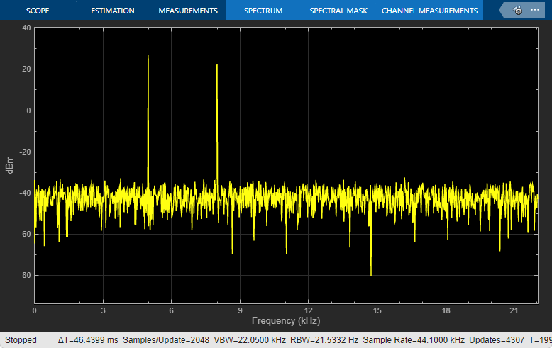
Run the model. The Spectrum Analyzer shows two tones at frequencies 5000 Hz and 10000 Hz, which correspond to the two frequencies at the input.

RBW, the resolution bandwidth is the minimum frequency bandwidth that can be resolved by the spectrum analyzer. By default, RBW (Hz) is set to Auto. In the Auto mode, RBW is the ratio of the frequency span to 1024. In a two-sided spectrum, this value is Fs/1024, while in a one-sided spectrum, it is (Fs/2)/1024. The spectrum analyzer in ex_psd_sa is configured to show one-sided spectrum. Hence, the RBW is (44100/2)/1024 or 21.53 Hz.
Using this value of RBW, the number of input samples used to compute one spectral update is given by Nsamples = Fs/RBW, which is 44100/21.53 or 2048.
RBW calculated in this mode gives a good frequency resolution.
To distinguish between two frequencies in the display, the distance between the two frequencies must be at least RBW. In this example, the distance between the two peaks is 5000 Hz, which is greater than RBW. Hence, you can see the peaks distinctly. Change the frequency of the second sine wave from 10000 Hz to 5015 Hz. The difference between the two frequencies is less than RBW.

On zooming, you can see that the peaks are not distinguishable.

To increase the frequency resolution, decrease RBW to 1 Hz and run the simulation. The two peaks, which are 15 Hz apart, are now distinguishable.

When you increase the frequency resolution, the time resolution decreases. To maintain a good balance between the frequency resolution and time resolution, change the RBW (Hz) to Auto.
Change the Input Signal
When you change the dynamics of the input signal during simulation, the power spectrum of the signal also changes in real time. While the simulation is running, change the Frequency of the Sine Wave 2 block to 8000 and click Apply. The second tone in the spectral analyzer output shifts to 8000 Hz and you can see the change in real time.

Change the Spectrum Analyzer Settings
When you change the settings in the Spectrum Analyzer block, the effect can be seen on the spectral data in real time.
When the model is running, in the Spectrum tab of the Spectrum Analyzer toolstrip, change the Frequency Scale to Log. The power spectrum is now displayed on a log scale.

For more information on how the Spectrum Analyzer settings affect the power spectrum data, see the 'Algorithms' section of the Spectrum Analyzer block reference page.
Estimate Power Spectrum Using the Spectrum Estimator Block
Alternately, you can compute the power spectrum of the signal using the Spectrum Estimator block in the dspspect3 library. You can acquire the output of the spectrum estimator and store the data for further processing.
Open and Run the Model
Replace the Spectrum Analyzer block in ex_psd_sa with the Spectrum Estimator block followed by an Array Plot block. Open the equivalent ex_psd_estimatorblock model. In addition, to access the spectral estimation data in MATLAB, connect the To Workspace (Simulink) block to the output of the Spectrum Estimator block.
The spectrum displayed in the Array Plot block is similar to the spectrum seen in the Spectrum Analyzer block in ex_psd_sa. The filter bank approach produces peaks that have very minimal spectral leakage.


Convert x-axis to Represent Frequency
By default, the Array Plot block plots the power spectrum data with respect to the number of samples per frame. The number of points on the x-axis equals the length of the input frame. The spectrum analyzer plots the power spectrum data with respect to frequency. For a one-sided spectrum, the frequency varies in the range [0 Fs/2]. For a two-sided spectrum, the frequency varies in the range [-Fs/2 Fs/2]. To convert the x-axis of the array plot from sample-based to frequency-based, do the following:
Click the Settings icon in the Scope tab of the Array Plot window. Under Data and Axes, set Sample Increment to Fs/FrameLength.
For a one-sided spectrum, set X-Offset to 0.
For a two-sided spectrum, set X-Offset to -Fs/2.
In this example, the spectrum is one-sided and hence, the Sample Increment and X-Offset are set to 44100/1024 and 0, respectively. To specify the frequency in kHz, set the Sample Increment to 44.1/1024.
Live Processing
The output of the Spectrum Estimator block contains the spectral data and is available for further processing. The data can be processed in real-time or it can be stored in the workspace using the To Workspace block. This example writes the spectral data to the workspace variable Estimate.