Train Neural ODE Network

This example shows how to train an augmented neural ordinary differential equation (ODE) network.

A neural ODE [1] is a deep learning operation that returns the solution of an ODE. In particular, given an input, a neural ODE operation outputs the numerical solution of the ODE $y' = f (t, y, θ)$ for the time horizon $(t_{0}, t_{1})$ and the initial condition $y (t_{0}) = y_{0}$ , where $t$ and $y$ denote the ODE function inputs and $θ$ is a set of learnable parameters. Typically, the initial condition $y_{0}$ is either the network input or, as in the case of this example, the output of another deep learning operation.

An augmented neural ODE [2] operation improves upon a standard neural ODE by augmenting the input data with extra channels and then discarding the augmentation after the neural ODE operation. Empirically, augmented neural ODEs are more stable, generalize better, and have a lower computational cost than neural ODEs.

This example trains a simple convolutional neural network with an augmented neural ODE operation.

The ODE function is itself a neural network. In this example, the model uses a network with a convolution and a tanh layer:

The example shows how to train a neural network to classify images of digits using an augmented neural ODE operation.

Load Training Data

Load the training images and labels using the digitTrain4DArrayData function.

load DigitsDataTrain

View the number of classes of the training data.

TTrain = labelsTrain;
classNames = categories(TTrain);
numClasses = numel(classNames)

numClasses = 10

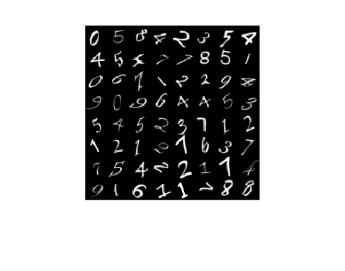
View some images from the training data.

numObservations = size(XTrain,4);
idx = randperm(numObservations,64);
I = imtile(XTrain(:,:,:,idx));
figure
imshow(I)

Define Neural Network Architecture

Define the following network, which classifies images.

A convolution-ReLU block with 8 3-by-3 filters with a stride of 2
An augmentation layer that concatenates an array of zeros to the input such that the output has twice as many channels as the input
A neural ODE operation with ODE function containing a convolution-tanh block with 16 3-by-3 filters
A discard augmentation layer that trims trailing elements in the channel dimension so that the output has half as many channels as the input
For classification output, a fully connect operation of size 10 (the number of classes) and a softmax operation

A neural ODE layer outputs the solution of a specified ODE function. For this example, specify a neural network that contains a convolution and tanh layer as the ODE function.

The neural ODE network must have matching input and output sizes. To calculate the input size of the neural network in the ODE layer, note that:

The input data for the image classification network are arrays of 28-by-28-by-1 images.
The images flow through a convolution layer with 8 filters that downsamples by a factor of 2.
The output of the convolution layer flows through an augmentation layer that doubles the number of channel dimensions.

This means that the inputs to the neural ODE layer are 14-by-14-by-16 arrays, where the spatial dimensions have size 14 and the channel dimension has size 16. Because the convolution layer downsamples the 28-by-28 images by a factor of two, the spatial sizes are 14. Because the convolution layer outputs 8 channels (the number of filters of the convolution layer) and that the augmentation layer doubles the number of channels, the channel size is 16.

Create the neural network to use for the neural ODE layer. Because the network does not have an input layer, do not initialize the network.

numFilters = 8;

layersODE = [
    convolution2dLayer(3,2*numFilters,Padding="same")
    tanhLayer];

netODE = dlnetwork(layersODE,Initialize=false);

Create the image classification network. For the augmentation and discard augmentation layers, use function layers with the channelAugmentation and discardChannelAugmentation functions listed in the Channel Augmentation Function and Discard Channel Augmentation Function sections of the example, respectively. To access these functions, open the example as a live script.

inputSize = size(XTrain,1:3);
filterSize = 3;
tspan = [0 0.1];

layers = [
    imageInputLayer(inputSize)
    convolution2dLayer(filterSize,numFilters)
    functionLayer(@channelAugmentation,Acceleratable=true,Formattable=true)
    neuralODELayer(netODE,tspan,GradientMode="adjoint")
    functionLayer(@discardChannelAugmentation,Acceleratable=true,Formattable=true)
    fullyConnectedLayer(numClasses)
    softmaxLayer];

Specify Training Options

Specify the training options. Choosing among the options requires empirical analysis. To explore different training option configurations by running experiments, you can use the Experiment Manager app.

Train using the Adam solver.
Train with a learning rate of 0.01.
Shuffle the data every epoch.
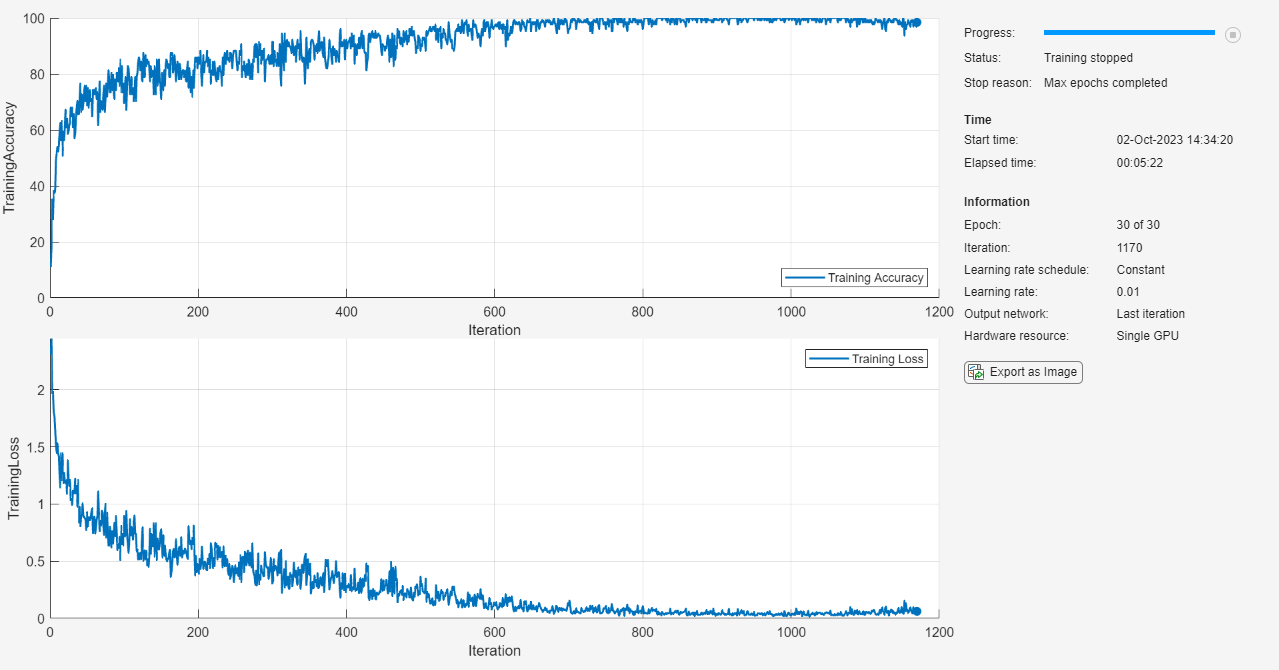
Monitor the training progress in a plot and display the accuracy.
Disable the verbose output.

options = trainingOptions("adam", ...
    InitialLearnRate=0.01, ...
    Shuffle="every-epoch", ...
    Plots="training-progress", ...
    Metrics="accuracy", ...
    Verbose=false);

Train the neural network using the trainnet function. For classification, use cross-entropy loss. By default, the trainnet function uses a GPU if one is available. Training on a GPU requires a Parallel Computing Toolbox™ license and a supported GPU device. For information on supported devices, see GPU Computing Requirements (Parallel Computing Toolbox). Otherwise, the trainnet function uses the CPU. To specify the execution environment, use the ExecutionEnvironment training option.

net = trainnet(XTrain,TTrain,layers,"crossentropy",options);

Test Model

Test the classification accuracy of the model by comparing the predictions on a held-out test set with the true labels.

Load the test data.

load DigitsDataTest
TTest = labelsTest;

Make predictions using the minibatchpredict function. To convert the prediction scores to labels, use the scores2label function. By default, the minibatchpredict function uses a GPU if one is available. Using a GPU requires a Parallel Computing Toolbox™ license and a supported GPU device. For information on supported devices, see GPU Computing Requirements (Parallel Computing Toolbox). Otherwise, the function uses the CPU. To specify the execution environment, use the ExecutionEnvironment option.

scores = minibatchpredict(net,XTest);
YTest = scores2label(scores,classNames);

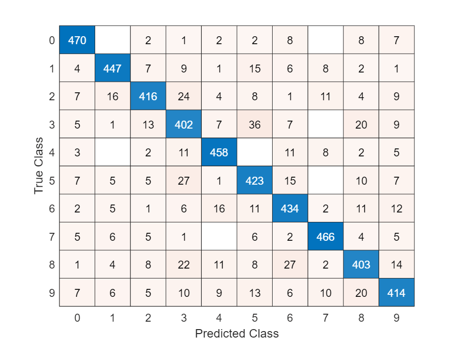
Visualize the predictions in a confusion matrix.

figure
confusionchart(TTest,YTest)

Calculate the classification accuracy.

accuracy = mean(TTest==YTest)

accuracy = 0.8666

Channel Augmentation Function

The channelAugmentation function augments pads the channel dimension of the input data X such that the output has twice as many channels.

function Z = channelAugmentation(X)

idxC = finddim(X,"C");
szC = size(X,idxC);
Z = paddata(X,2*szC,Dimension=idxC);

end

Discard Channel Augmentation Function

The discardChannelAugmentation function augments trims the channel dimension of the input data X such that the output has half as many channels.

function Z = discardChannelAugmentation(X)

idxC = finddim(X,"C");
szC = size(X,idxC);
Z = trimdata(X,floor(szC/2),Dimension=idxC);

end

Bibliography

Chen, Ricky T. Q., Yulia Rubanova, Jesse Bettencourt, and David Duvenaud. “Neural Ordinary Differential Equations.” Preprint, submitted June 19, 2018. https://arxiv.org/abs/1806.07366.
Dupont, Emilien, Arnaud Doucet, and Yee Whye Teh. “Augmented Neural ODEs.” Preprint, submitted October 26, 2019. https://arxiv.org/abs/1904.01681.