Backtest Strategies Using Deep Learning
Construct trading strategies using a deep learning model and then backtest the strategies using the Financial Toolbox™ backtesting framework. The example uses Deep Learning Toolbox™ to train a predictive model from a set of time series and demonstrates the steps necessary to convert the model output into trading signals. It builds a variety of trading strategies that backtest the signal data over a 5-year period.
This example illustrates the following workflow:
The focus of this example is on the workflow from data, to a trained model, to trading strategies, and finally to a backtest of the strategies. The deep learning model, its output, the subsequent trading signals, and the strategies are fictional. The intent is only to show the steps for developing and deploying this type of model.
Load Data
Load the historical price data. This data set contains daily spot prices for 12 different energy products ranging from 1986 to 2021 and consists of the following time series:
WTI — West Texas Intermediate light crude oil
Brent — Brent light crude oil
NaturalGas — Henry Hub natural gas
Propane — Mon Belvieu propane
Kerosene — US Gulf Coast kerosene-type jet fuel
HeatingOil — New York Harbor no. 2 heating oil
GulfRegular — US Gulf Coast conventional gasoline
LARegular — Los Angeles reformulated RBOB regular gasoline
NYRegular — New York Harbor conventional gasoline
GulfDiesel — US Gulf Coast ultra-low sulfur no. 2 diesel
LADiesel — Los Angeles ultra-low sulfur CARB diesel
NYDiesel — New York Harbor ultra-low sulfur no. 2 diesel
The source of this data is the US Energy Information Administration (Nov 2021).
priceData = load('energyPrices.mat','energyPrices');
priceData = priceData.energyPrices;
tail(priceData)
       Time         WTI     Brent    NaturalGas    Propane    Kerosene    HeatingOil    GulfRegular    LARegular    NYRegular    GulfDiesel    LADiesel    NYDiesel
    ___________    _____    _____    __________    _______    ________    __________    ___________    _________    _________    __________    ________    ________

    22-Oct-2021    84.53    85.43        5.1        1.485      2.312        2.414          2.481         2.671        2.571         2.49        2.559       2.558
    25-Oct-2021    84.64    84.85       5.72        1.378      2.326        2.429          2.506         2.691        2.591        2.501        2.573       2.572
    26-Oct-2021    85.64    85.11       5.59        1.398      2.339        2.436          2.552         2.636        2.591        2.511        2.598       2.573
    27-Oct-2021    82.66    84.12       5.91        1.365      2.271        2.368          2.469         2.566        2.508        2.443        2.535       2.505
    28-Oct-2021    82.78     83.4       5.68         1.36      2.278        2.363          2.471         2.583        2.518        2.448         2.57        2.51
    29-Oct-2021     83.5     83.1       5.49        1.383      2.285        2.342          2.485         2.662        2.537        2.429        2.573       2.487
    01-Nov-2021    84.08    84.51       5.22        1.385      2.301        2.364          2.457         2.597        2.494        2.445        2.599       2.511
    02-Nov-2021    83.91    84.42       5.33        1.388        2.3        2.405          2.466         2.601        2.596        2.441        2.595        2.51
Clean and Trim Data
The price datasets do not all start at the same time. Some datasets start later than others and have fewer data points. The following plot shows the time span for each price series.
seriesLifespanPlot(priceData)
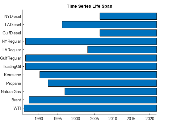
To avoid large spans of missing data, remove the series with shorter histories.
priceData = removevars(priceData,["NYDiesel","GulfDiesel","LARegular"]);
The remaining table variables contain sporadic missing elements (NaNs) due to holidays or other reasons. Missing data is handled in a variety of ways depending on the dataset. In some cases, it may be appropriate to interpolate or use the fillmissing function. In this example, you can remove the remaining NaN prices.
priceData = rmmissing(priceData);
Then, convert the price data to a return series using the tick2ret (Financial Toolbox) function. The final dataset consists of nine price series with daily data from 1997 through 2021.
returnData = tick2ret(priceData)
returnData=6167×9 timetable
    08-Jan-1997     0.0114     8.0775e-04    -0.0052          0     0.0129     0.0110     0.0014    -0.0028    -0.0066
    09-Jan-1997    -0.0094         0.0020    -0.0500    -0.0370    -0.0085    -0.0014    -0.0244    -0.0242          0
    10-Jan-1997    -0.0057        -0.0246     0.0859     0.0096    -0.0100    -0.0122    -0.0088    -0.0058    -0.0093
    13-Jan-1997    -0.0363        -0.0334     0.0204    -0.0247    -0.0347    -0.0371    -0.0296    -0.0367    -0.0067
    15-Jan-1997     0.0298        -0.0043     0.0850    -0.0487     0.0240     0.0214     0.0031     0.0061    -0.0135
    16-Jan-1997    -0.0193              0     0.0853    -0.0287    -0.0190    -0.0210     0.0061     0.0030     0.0205
    17-Jan-1997    -0.0020        -0.0189    -0.1699    -0.0169    -0.0209    -0.0200    -0.0061    -0.0075          0
    20-Jan-1997    -0.0118    -4.3725e-04    -0.1662    -0.0279    -0.0228    -0.0219     0.0015    -0.0137    -0.0040
    21-Jan-1997    -0.0120         0.0052    -0.0828    -0.0044    -0.0140    -0.0209     0.0213     0.0123    -0.0067
    22-Jan-1997    -0.0161        -0.0022     0.0201    -0.0044     0.0316     0.0198     0.0134     0.0167          0
    23-Jan-1997    -0.0225              0    -0.0295    -0.0022    -0.0061    -0.0119    -0.0352     0.0105     0.0405
    24-Jan-1997          0        -0.0057    -0.1149    -0.0759     0.0108     0.0060     0.0061    -0.0089     0.0065
    27-Jan-1997          0        -0.0105     0.1374     0.0169     0.0122     0.0090     0.0030    -0.0030     0.0297
    28-Jan-1997     0.0021         0.0027     0.0235    -0.0048     0.0090    -0.0089    -0.0106    -0.0120     0.0439
      ⋮
Prepare Data for Training LSTM Model
Prepare and partition the dataset in order to train the LSTM model. The model uses a 30-day rolling window of trailing feature data and predicts the next day price changes for four of the assets: Brent crude oil, natural gas, propane, and kerosene.
% Model is trained using a 30-day rolling window to predict 1 day in the
% future.
historySize = 30;
futureSize = 1;

% Model predicts returns for oil, natural gas, propane, and kerosene.
outputVarName = ["Brent" "NaturalGas", "Propane" "Kerosene"];
numOutputs = numel(outputVarName);

% start_idx and end_idx are the index positions in the returnData
% timetable corresponding to the first and last date for making a prediction.
start_idx = historySize + 1;
end_idx   = height(returnData) - futureSize + 1;
numSamples = end_idx - start_idx + 1;

% The date_vector variable stores the dates for making predictions.
date_vector = returnData.Time(start_idx-1:end_idx-1);
Convert the returnData timetable to a numSamples-by-1 cell array. Each cell contains a numFeatures-by-seqLength matrix. The response variable is a numSamples-by-numResponses matrix.
network_features  = cell(numSamples,1);
network_responses = zeros(numSamples,numOutputs);

for j = 1:numSamples
    network_features{j} = (returnData(j:j+historySize-1,:).Variables)';
    network_responses(j,:) = ...
        (returnData(j+historySize:j+historySize+futureSize-1,outputVarName).Variables)';
end
Split the network_features and the network_responses into three parts: training, validation, and backtesting. Select the backtesting set as a set of sequential data points. The remainder of the data is randomly split into a training and a validation set. Use the validation set to prevent overfitting while training the model. The backtesting set is not used in the training process, but it is reserved for the final strategy backtest.
% Specify rows to use in the backtest (31-Dec-2015 to 2-Nov-2021).
backtest_start_idx = find(date_vector < datetime(2016,1,1),1,'last');
backtest_indices = backtest_start_idx:size(network_responses,1);

% Specify data reserved for the backtest.
Xbacktest = network_features(backtest_indices);
Tbacktest = network_responses(backtest_indices,:);

% Remove the backtest data.
network_features = network_features(1:backtest_indices(1)-1);
network_responses = network_responses(1:backtest_indices(1)-1,:);

% Partition the remaining data into training and validation sets.
rng('default');
cv_partition = cvpartition(size(network_features,1),'HoldOut',0.2);

% Training set
Xtraining = network_features(~cv_partition.test,:);
Ttraining = network_responses(~cv_partition.test,:);

% Validation set
Xvalidation = network_features(cv_partition.test,:);
Tvalidation = network_responses(cv_partition.test,:);
Define LSTM Network Architecture
Specify the network architecture as a series of layers. For more information on LSTM networks, see Long Short-Term Memory Neural Networks. The Deep Network Designer is a powerful tool for designing deep learning models.
numFeatures = width(returnData);
numHiddenUnits_LSTM = 10;

layers_LSTM = [ ...
    sequenceInputLayer(numFeatures)
    lstmLayer(numHiddenUnits_LSTM)
    layerNormalizationLayer
    lstmLayer(numHiddenUnits_LSTM)
    layerNormalizationLayer
    lstmLayer(numHiddenUnits_LSTM,'OutputMode','last')
    layerNormalizationLayer
    fullyConnectedLayer(numOutputs)];
Specify Training Options for LSTM Model
Next, you specify training options using the trainingOptions function. Many training options are available and their use varies depending on your use case. Use the Experiment Manager to explore different network architectures and sets of network hyperparameters.
max_epochs = 500;
mini_batch_size = 128;
learning_rate = 1e-4;

options_LSTM = trainingOptions('adam', ...
    'InputDataFormats',"CTB",...
    'Plots','training-progress', ...
    'Verbose',0, ...
    'MaxEpochs',max_epochs, ...
    'MiniBatchSize',mini_batch_size, ...
    'Shuffle','every-epoch', ...
    'ValidationData',{Xvalidation,Tvalidation}, ...
    'ValidationFrequency',50, ...
    'ValidationPatience',10, ...
    'InitialLearnRate',learning_rate, ...
    'GradientThreshold',1);
Train LSTM Model
Train the LSTM network. Use the trainNetwork function to train the network until the network meets a stopping criteria. This process can take several minutes depending on the computer running the example. For more information on increasing the network training performance, see Scale Up Deep Learning in Parallel, on GPUs, and in the Cloud.
To avoid waiting for the network training, load the pretrained network by setting the doTrain flag to false. To train the network using trainNetwork, set the doTrain flag to true.
doTrain = false;

if doTrain
    % Train the LSTM network.
    net_LSTM = trainnet(Xtraining,Ttraining,layers_LSTM,"mse",options_LSTM);
else
    % Load the pretrained network.
    load lstmBacktestNetwork
end
Visualize Training Results
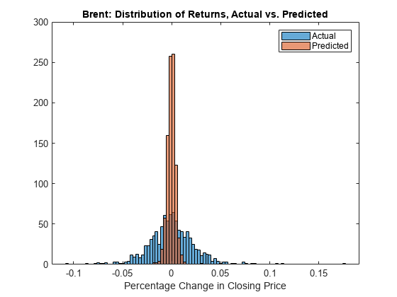
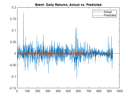
Visualize the results of the trained model by comparing the predicted values against the actual values from the validation set.
% Compare the actual returns to model predicted returns.
actual    = Tvalidation;
predicted = minibatchpredict(net_LSTM,Xvalidation,InputDataFormats="CTB");
% Overlay histogram of actual vs. predicted returns for the validation set. output_idx =1; figure; [~,edges] = histcounts(actual(:,output_idx),100); histogram(actual(:,output_idx),edges); hold on histogram(predicted(:,output_idx),edges) hold off xlabel('Percentage Change in Closing Price') legend('Actual','Predicted') title(sprintf('%s: Distribution of Returns, Actual vs. Predicted', outputVarName(output_idx)))
% Display the predicted vs. actual daily returns for the validation set.
figure
plot(actual(:,output_idx))
hold on
plot(predicted(:,output_idx))
yline(0)
legend({'Actual','Predicted'})
title(sprintf('%s: Daily Returns, Actual vs. Predicted', outputVarName(output_idx)))
% Examine the residuals.
residuals = actual(:,output_idx) - predicted(:,output_idx);
figure;
normplot(residuals);
The actual data has fatter tails than the trained model predictions. The model predictions are not accurate, but the goal of this example is to show the workflow from loading data, to model development, to backtesting. A more sophisticated model with a larger and more varied set of training data is likely to have more predictive power.
Prepare Backtest Data
Use the predictions from the LSTM model to build the backtest strategies. You can post-process the model output in a number of ways to create trading signals. However, for this example, take the model regression output and convert it to a timetable.
Use predict with the trained network to generate model predictions over the backtest period.
backtestPred_LSTM = minibatchpredict(net_LSTM,Xbacktest,InputDataFormats="CTB");Convert the predictions to a trading signal timetable.
backtestSignalTT = timetable(date_vector(backtest_indices),backtestPred_LSTM);
Construct the prices timetable corresponding to the backtest time span. The backtest trades in and out of the four energy commodities. The prices timetable has the closing price for the day on which the prediction is made.
backtestPriceTT = priceData(date_vector(backtest_indices),outputVarName);
Set the risk-free rate to be 1% annualized. The backtest engine also supports setting the risk-free rate to a timetable containing the historical daily rates.
risk_free_rate = 0.01;
Create Backtest Strategies
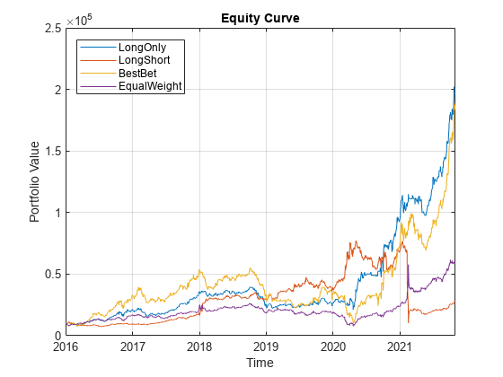
Use backtestStrategy (Financial Toolbox) to create four trading strategies based on the signal indicators. The following trading strategies are intended as examples to show how to convert the trading signals into actionable asset allocation strategies that you can then backtest:
Long Only — Invest all capital across the assets with positive predicted return, proportional to their signal strength (predicted return).
Long Short — Invest capital across the assets, both long and short positions, proportional to their signal strength.
Best Bet — Invest all capital into the single asset with the highest predicted return.
Equal Weight — Rebalance each day to equal-weighted allocation.
% Specify 10 basis points as the trading cost.
tradingCosts = 0.001;

% Invest in long positions proportionally to their predicted return.
LongStrategy = backtestStrategy('LongOnly',@LongOnlyRebalanceFcn, ...
    'TransactionCosts',tradingCosts, ...
    'LookbackWindow',1);

% Invest in both long and short positions proportionally to their predicted returns.
LongShortStrategy = backtestStrategy('LongShort',@LongShortRebalanceFcn, ...
    'TransactionCosts',tradingCosts, ...
    'LookbackWindow',1);

% Invest 100% of capital into single asset with highest predicted returns.
BestBetStrategy = backtestStrategy('BestBet',@BestBetRebalanceFcn, ...
    'TransactionCosts',tradingCosts, ...
    'LookbackWindow',1);

% For comparison, invest in an equal-weighted (buy low and sell high) strategy.
equalWeightFcn = @(current_weights,prices,signal) ones(size(current_weights)) / numel(current_weights);
EqualWeightStrategy = backtestStrategy('EqualWeight',equalWeightFcn, ...
    'TransactionCosts',tradingCosts, ...
    'LookbackWindow',0);
Put the strategies into an array and then use backtestEngine (Financial Toolbox) to create the backtesting engine.
strategies = [LongStrategy LongShortStrategy BestBetStrategy EqualWeightStrategy];

bt = backtestEngine(strategies,'RiskFreeRate',risk_free_rate);
Run Backtest
Use runBacktest (Financial Toolbox) to backtest the strategies over the backtest range.
bt = runBacktest(bt,backtestPriceTT,backtestSignalTT)
bt =
  backtestEngine with properties:

               Strategies: [1×4 backtestStrategy]
             RiskFreeRate: 0.0100
           CashBorrowRate: 0
          RatesConvention: "Annualized"
                    Basis: 0
    InitialPortfolioValue: 10000
           DateAdjustment: "Previous"
      PayExpensesFromCash: 0
                NumAssets: 4
                  Returns: [1462×4 timetable]
                Positions: [1×1 struct]
                 Turnover: [1462×4 timetable]
                  BuyCost: [1462×4 timetable]
                 SellCost: [1462×4 timetable]
         TransactionCosts: [1×1 struct]
                     Fees: [1×1 struct]
Examine Backtest Results
Use the summary (Financial Toolbox) and equityCurve (Financial Toolbox) functions to summarize and plot the backtest results. This model and its derivative trading strategies are not expected to be profitable in a realistic trading scenario. However, this example illustrates a workflow that should be useful for practitioners with more comprehensive data sets and more sophisticated models and strategies.
summary(bt)
ans=9×4 table
    18.6523    1.8281    17.6515    4.8347
     0.0858    0.0398     0.0706    0.0568
     0.0277    0.0335     0.0377    0.0267
     0.2372    0.2888     0.2596    0.0096
          1    1.3867          1    0.5000
     0.0024    0.0014     0.0027    0.0016
     0.4666    0.8660     0.8256    0.7051
    10.3149    8.3730    11.3932    0.2026
    10.4449    8.4198    11.3864    0.1958
figure;
equityCurve(bt)
Local Functions
function new_weights = LongOnlyRebalanceFcn(current_weights,pricesTT,signalTT)
% Long only strategy, in proportion to the signal.

signal = signalTT.backtestPred_LSTM(end,:);

if any(0 < signal)
    signal(signal < 0) = 0;
    new_weights = signal / sum(signal);
else
    new_weights = zeros(size(current_weights));
end

end


function new_weights = LongShortRebalanceFcn(current_weights,pricesTT,signalTT) %#ok<INUSD>
% Long/Short strategy, in proportion to the signal

signal = signalTT.backtestPred_LSTM(end,:);
abssum = sum(abs(signal));

if 0 < abssum
    new_weights = signal / abssum;
else
    new_weights = zeros(size(current_weights));
end

end


function new_weights = BestBetRebalanceFcn(current_weights,pricesTT,signalTT) %#ok<INUSD>
% Best bet strategy, invest in the asset with the most upside.

signal = signalTT.backtestPred_LSTM(end,:);
new_weights = zeros(size(current_weights));
new_weights(signal == max(signal)) = 1;

end


function seriesLifespanPlot(priceData)
% Plot the lifespan of each time series.

% Specify all time series end on same day.
d2 = numel(priceData.Time);

% Plot the lifespan patch for each series.
numSeries = size(priceData,2);
for i = 1:numSeries
    % Find start date index.
    d1 = find(~isnan(priceData{:,i}),1,'first');
    % Plot patch.
    x = [d1 d1 d2 d2];
    y = i + [-0.4 0.4 0.4 -0.4];
    patch(x,y,[0 0.4470 0.7410])

    hold on
end
hold off

% Set the plot properties.
xlim([-100 d2]);
ylim([0.2 numSeries + 0.8]);

yticks(1:numSeries);
yticklabels(priceData.Properties.VariableNames');
flipud(gca);

years = 1990:5:2021;
xtick_idx = zeros(size(years));
for yidx = 1:numel(years)
    xtick_idx(yidx) = find(years(yidx) == year(priceData.Time),1,'first');
end
xticks(xtick_idx);
xticklabels(string(years));

title('Time Series Life Span');

end
See Also
Deep Network Designer | trainnet | trainingOptions | dlnetwork | backtestStrategy (Financial Toolbox) | backtestEngine (Financial Toolbox) | runBacktest (Financial Toolbox) | equityCurve (Financial Toolbox) | summary (Financial Toolbox)
Topics
- Backtest Investment Strategies Using Financial Toolbox (Financial Toolbox)
- Backtest Investment Strategies with Trading Signals (Financial Toolbox)
- Backtest Using Risk-Based Equity Indexation (Financial Toolbox)
- Backtest Strategies Using Deep Learning (Financial Toolbox)