Main Content

squeezenet

SqueezeNet convolutional neural network

  • SqueezeNet network architecture

Description

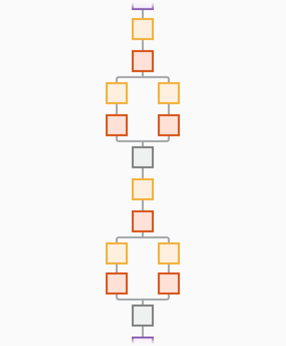
SqueezeNet is a convolutional neural network that is 18 layers deep. You can load a pretrained version of the network trained on more than a million images from the ImageNet database [1]. The pretrained network can classify images into 1000 object categories, such as keyboard, mouse, pencil, and many animals. As a result, the network has learned rich feature representations for a wide range of images. This function returns a SqueezeNet v1.1 network, which has similar accuracy to SqueezeNet v1.0 but requires fewer floating-point operations per prediction [3]. The network has an image input size of 227-by-227. For more pretrained networks in MATLAB®, see Pretrained Deep Neural Networks.

You can use classify to classify new images using the SqueezeNet network. For an example, see Classify Image Using SqueezeNet.

You can retrain a SqueezeNet network to perform a new task using transfer learning. For an example, see Interactive Transfer Learning Using SqueezeNet.

example

net = squeezenet returns a SqueezeNet network trained on the ImageNet data set.

net = squeezenet('Weights','imagenet') returns a SqueezeNet network trained on the ImageNet data set. This syntax is equivalent to net = squeezenet.

lgraph = squeezenet('Weights','none') returns the untrained SqueezeNet network architecture.

Examples

collapse all

Load a pretrained SqueezeNet network.

net = squeezenet
net = 

  DAGNetwork with properties:

         Layers: [68×1 nnet.cnn.layer.Layer]
    Connections: [75×2 table]

This function returns a DAGNetwork object.

SqueezeNet is included within Deep Learning Toolbox™. To load other networks, use functions such as googlenet to get links to download pretrained networks from the Add-On Explorer.

This example shows how to fine-tune a pretrained SqueezeNet network to classify a new collection of images. This process is called transfer learning and is usually much faster and easier than training a new network, because you can apply learned features to a new task using a smaller number of training images. To prepare a network for transfer learning interactively, use Deep Network Designer.

Extract Data

In the workspace, extract the MathWorks Merch data set. This is a small data set containing 75 images of MathWorks merchandise, belonging to five different classes (cap, cube, playing cards, screwdriver, and torch).

unzip("MerchData.zip");

Open SqueezeNet in Deep Network Designer

Open Deep Network Designer with SqueezeNet.

deepNetworkDesigner(squeezenet);

Deep Network Designer displays a zoomed-out view of the whole network in the Designer pane.

Explore the network plot. To zoom in with the mouse, use Ctrl+scroll wheel. To pan, use the arrow keys, or hold down the scroll wheel and drag the mouse. Select a layer to view its properties. Deselect all layers to view the network summary in the Properties pane.

Import Data

To load the data into Deep Network Designer, on the Data tab, click Import Data > Import Image Classification Data.

In the Data source list, select Folder. Click Browse and select the extracted MerchData folder.

Divide the data into 70% training data and 30% validation data.

Specify augmentation operations to perform on the training images. For this example, apply a random reflection in the x-axis, a random rotation from the range [-90,90] degrees, and a random rescaling from the range [1,2]. Data augmentation helps prevent the network from overfitting and memorizing the exact details of the training images.

Click Import to import the data into Deep Network Designer.

Visualize Data

Using Deep Network Designer, you can visually inspect the distribution of the training and validation data in the Data tab. You can also view random observations and their labels as a simple check before training. You can see that, in this example, there are five classes in the data set.

Edit Network for Transfer Learning

The convolutional layers of the network extract image features that the last learnable layer and the final classification layer use to classify the input image. These two layers, 'conv10' and 'ClassificationLayer_predictions' in SqueezeNet, contain information on how to combine the features that the network extracts into class probabilities, a loss value, and predicted labels. To retrain a pretrained network to classify new images, adapt these two layers to the new data set.

To use a pretrained network for transfer learning, you must change the number of classes to match your new data set. First, select the 'conv10' layer. At the bottom of the Properties pane, click Unlock Layer. In the warning dialog that appears, click Unlock Anyway. This unlocks the layer properties so that you can adapt them to your new task.

Before R2023b: To edit the layer properties, you must replace the layers instead of unlocking them. In the new convolutional 2-D layer, set the FilterSize to [1 1].

The NumFilters property defines the number of classes for classification problems. Change NumFilters to the number of classes in the new data, in this example, 5.

Change the learning rates so that learning is faster in the new layer than in the transferred layers by setting WeightLearnRateFactor and BiasLearnRateFactor to 10.

Next, configure the output layer. Select the final classification layer, ClassificationLayer_predictions, and click Unlock Layer and then click Unlock Anyway. For the unlocked output layer, you do not need to set the OutputSize. At training time, Deep Network Designer automatically sets the output classes of the layer from the data.

Check Network

To make sure your edited network is ready for training, click Analyze, and ensure the Deep Learning Network Analyzer reports zero errors.

Train Network

Specify training options. Select the Training tab and click Training Options.

  • Set the initial learn rate to a small value to slow down learning in the transferred layers.

  • Specify the validation frequency so that the accuracy on the validation data is calculated once every epoch.

  • Specify a small number of epochs. An epoch is a full training cycle on the entire training data set. For transfer learning, you do not need to train for as many epochs.

  • Specify the mini-batch size, that is, how many images to use in each iteration. To ensure the whole data set is used during each epoch, set the mini-batch size to evenly divide the number of training samples.

For this example, set InitialLearnRate to 0.0001, MaxEpochs to 8, and ValidationFrequency to 5. As there are 55 observations, set MiniBatchSize to 11.

To train the network with the specified training options, click OK and then click Train.

Deep Network Designer allows you to visualize and monitor training progress. You can then edit the training options and retrain the network, if required.

Export Results and Generate MATLAB Code

To export the network architecture with the trained weights, on the Training tab, select Export > Export Trained Network and Results. Deep Network Designer exports the trained network as the variable trainedNetwork_1 and the training info as the variable trainInfoStruct_1.

You can also generate MATLAB code, which recreates the network and the training options used. On the Training tab, select Export > Generate Code for Training. Examine the MATLAB code to learn how to programmatically prepare the data for training, create the network architecture, and train the network.

Classify New Image

Load a new image to classify using the trained network.

I = imread("MerchDataTest.jpg");

Deep Network Designer resizes the images during training to match the network input size. To view the network input size, go to the Designer pane and select the imageInputLayer (first layer). This network has an input size of 227-by-227.

Resize the test image to match the network input size.

I = imresize(I, [227 227]);

Classify the test image using the trained network.

[YPred,probs] = classify(trainedNetwork_1,I);
imshow(I)
label = YPred;
title(string(label) + ", " + num2str(100*max(probs),3) + "%");

This example shows how to fine-tune a pretrained SqueezeNet convolutional neural network to perform classification on a new collection of images.

SqueezeNet has been trained on over a million images and can classify images into 1000 object categories (such as keyboard, coffee mug, pencil, and many animals). The network has learned rich feature representations for a wide range of images. The network takes an image as input and outputs a label for the object in the image together with the probabilities for each of the object categories.

Transfer learning is commonly used in deep learning applications. You can take a pretrained network and use it as a starting point to learn a new task. Fine-tuning a network with transfer learning is usually much faster and easier than training a network with randomly initialized weights from scratch. You can quickly transfer learned features to a new task using a smaller number of training images.

Load Data

Unzip and load the new images as an image datastore. imageDatastore automatically labels the images based on folder names and stores the data as an ImageDatastore object. An image datastore enables you to store large image data, including data that does not fit in memory, and efficiently read batches of images during training of a convolutional neural network.

unzip('MerchData.zip');
imds = imageDatastore('MerchData', ...
    'IncludeSubfolders',true, ...
    'LabelSource','foldernames');

Divide the data into training and validation data sets. Use 70% of the images for training and 30% for validation. splitEachLabel splits the images datastore into two new datastores.

[imdsTrain,imdsValidation] = splitEachLabel(imds,0.7,'randomized');

This very small data set now contains 55 training images and 20 validation images. Display some sample images.

numTrainImages = numel(imdsTrain.Labels);
idx = randperm(numTrainImages,16);

I = imtile(imds, 'Frames', idx);

figure
imshow(I)

Figure contains an axes object. The axes object contains an object of type image.

Load Pretrained Network

Load the pretrained SqueezeNet neural network.

net = squeezenet;

Use analyzeNetwork to display an interactive visualization of the network architecture and detailed information about the network layers.

analyzeNetwork(net)

The first layer, the image input layer, requires input images of size 227-by-227-by-3, where 3 is the number of color channels.

inputSize = net.Layers(1).InputSize
inputSize = 1×3

   227   227     3

Replace Final Layers

The convolutional layers of the network extract image features that the last learnable layer and the final classification layer use to classify the input image. These two layers, 'conv10' and 'ClassificationLayer_predictions' in SqueezeNet, contain information on how to combine the features that the network extracts into class probabilities, a loss value, and predicted labels. To retrain a pretrained network to classify new images, replace these two layers with new layers adapted to the new data set.

Extract the layer graph from the trained network.

lgraph = layerGraph(net); 

Find the names of the two layers to replace. You can do this manually or you can use the supporting function findLayersToReplace to find these layers automatically.

[learnableLayer,classLayer] = findLayersToReplace(lgraph);
[learnableLayer,classLayer] 
ans = 
  1x2 Layer array with layers:

     1   'conv10'                            2-D Convolution         1000 1x1x512 convolutions with stride [1  1] and padding [0  0  0  0]
     2   'ClassificationLayer_predictions'   Classification Output   crossentropyex with 'tench' and 999 other classes

In most networks, the last layer with learnable weights is a fully connected layer. In some networks, such as SqueezeNet, the last learnable layer is a 1-by-1 convolutional layer instead. In this case, replace the convolutional layer with a new convolutional layer with the number of filters equal to the number of classes. To learn faster in the new layers than in the transferred layers, increase the WeightLearnRateFactor and BiasLearnRateFactor values of the convolutional layer.

numClasses = numel(categories(imdsTrain.Labels))
numClasses = 5
newConvLayer =  convolution2dLayer([1, 1],numClasses,'WeightLearnRateFactor',10,'BiasLearnRateFactor',10,"Name",'new_conv');
lgraph = replaceLayer(lgraph,'conv10',newConvLayer);

The classification layer specifies the output classes of the network. Replace the classification layer with a new one without class labels. trainNetwork automatically sets the output classes of the layer at training time.

newClassificatonLayer = classificationLayer('Name','new_classoutput');
lgraph = replaceLayer(lgraph,'ClassificationLayer_predictions',newClassificatonLayer);

Train Network

The network requires input images of size 227-by-227-by-3, but the images in the image datastores have different sizes. Use an augmented image datastore to automatically resize the training images. Specify additional augmentation operations to perform on the training images: randomly flip the training images along the vertical axis, and randomly translate them up to 30 pixels horizontally and vertically. Data augmentation helps prevent the network from overfitting and memorizing the exact details of the training images.

pixelRange = [-30 30];
imageAugmenter = imageDataAugmenter( ...
    'RandXReflection',true, ...
    'RandXTranslation',pixelRange, ...
    'RandYTranslation',pixelRange);
augimdsTrain = augmentedImageDatastore(inputSize(1:2),imdsTrain, ...
    'DataAugmentation',imageAugmenter);

To automatically resize the validation images without performing further data augmentation, use an augmented image datastore without specifying any additional preprocessing operations.

augimdsValidation = augmentedImageDatastore(inputSize(1:2),imdsValidation);

Specify the training options. For transfer learning, keep the features from the early layers of the pretrained network (the transferred layer weights). To slow down learning in the transferred layers, set the initial learning rate to a small value. In the previous step, you increased the learning rate factors for the convolutional layer to speed up learning in the new final layers. This combination of learning rate settings results in fast learning only in the new layers and slower learning in the other layers. When performing transfer learning, you do not need to train for as many epochs. An epoch is a full training cycle on the entire training data set. Specify the mini-batch size to be 11 so that in each epoch you consider all of the data. The software validates the network every ValidationFrequency iterations during training.

options = trainingOptions('sgdm', ...
    'MiniBatchSize',11, ...
    'MaxEpochs',7, ...
    'InitialLearnRate',2e-4, ...
    'Shuffle','every-epoch', ...
    'ValidationData',augimdsValidation, ...
    'ValidationFrequency',3, ...
    'Verbose',false, ...
    'Plots','training-progress');

Train the network that consists of the transferred and new layers. By default, trainNetwork uses a GPU if one is available. This requires Parallel Computing Toolbox™ and a supported GPU device. For information on supported devices, see GPU Computing Requirements (Parallel Computing Toolbox). Otherwise, trainNetwork uses a CPU. You can also specify the execution environment by using the 'ExecutionEnvironment' name-value pair argument of trainingOptions.

netTransfer = trainNetwork(augimdsTrain,lgraph,options);

Figure Training Progress (19-Aug-2023 11:48:09) contains 2 axes objects and another object of type uigridlayout. Axes object 1 with xlabel Iteration, ylabel Loss contains 14 objects of type patch, text, line. Axes object 2 with xlabel Iteration, ylabel Accuracy (%) contains 14 objects of type patch, text, line.

Classify Validation Images

Classify the validation images using the fine-tuned network.

[YPred,scores] = classify(netTransfer,augimdsValidation);

Display four sample validation images with their predicted labels.

idx = randperm(numel(imdsValidation.Files),4);
figure
for i = 1:4
    subplot(2,2,i)
    I = readimage(imdsValidation,idx(i));
    imshow(I)
    label = YPred(idx(i));
    title(string(label));
end

Figure contains 4 axes objects. Axes object 1 with title MathWorks Playing Cards contains an object of type image. Axes object 2 with title MathWorks Playing Cards contains an object of type image. Axes object 3 with title MathWorks Cube contains an object of type image. Axes object 4 with title MathWorks Cube contains an object of type image.

Calculate the classification accuracy on the validation set. Accuracy is the fraction of labels that the network predicts correctly.

YValidation = imdsValidation.Labels;
accuracy = mean(YPred == YValidation)
accuracy = 1

For tips on improving classification accuracy, see Deep Learning Tips and Tricks.

Read, resize, and classify an image using SqueezeNet.

First, load a pretrained SqueezeNet model.

net = squeezenet;

Read the image using imread.

I = imread('peppers.png');
figure
imshow(I)

Figure contains an axes object. The axes object contains an object of type image.

The pretrained model requires the image size to be the same as the input size of the network. Determine the input size of the network using the InputSize property of the first layer of the network.

sz = net.Layers(1).InputSize
sz = 1×3

   227   227     3

Resize the image to the input size of the network.

I = imresize(I,sz(1:2));
figure
imshow(I)

Figure contains an axes object. The axes object contains an object of type image.

Classify the image using classify.

label = classify(net,I)
label = categorical
     bell pepper 

Show the image and classification result together.

figure
imshow(I)
title(label)

Figure contains an axes object. The axes object with title bell pepper contains an object of type image.

This example shows how to extract learned image features from a pretrained convolutional neural network and use those features to train an image classifier.

Feature extraction is the easiest and fastest way to use the representational power of pretrained deep networks. For example, you can train a support vector machine (SVM) using fitcecoc (Statistics and Machine Learning Toolbox™) on the extracted features. Because feature extraction requires only a single pass through the data, it is a good starting point if you do not have a GPU to accelerate network training with.

Load Data

Unzip and load the sample images as an image datastore. imageDatastore automatically labels the images based on folder names and stores the data as an ImageDatastore object. An image datastore lets you store large image data, including data that does not fit in memory. Split the data into 70% training and 30% test data.

unzip("MerchData.zip");

imds = imageDatastore("MerchData", ...
    IncludeSubfolders=true, ...
    LabelSource="foldernames");

[imdsTrain,imdsTest] = splitEachLabel(imds,0.7,"randomized");

This very small data set now has 55 training images and 20 validation images. Display some sample images.

numImagesTrain = numel(imdsTrain.Labels);
idx = randperm(numImagesTrain,16);

I = imtile(imds,"Frames",idx);

figure
imshow(I)

Load Pretrained Network

Load a pretrained SqueezeNet network. SqueezeNet is trained on more than a million images and can classify images into 1000 object categories, for example, keyboard, mouse, pencil, and many animals. As a result, the model has learned rich feature representations for a wide range of images.

net = squeezenet;

Analyze the network architecture.

analyzeNetwork(net)

2022-01-07_16-31-30.png

The first layer, the image input layer, requires input images of size 227-by-227-by-3, where 3 is the number of color channels.

inputSize = net.Layers(1).InputSize
inputSize = 1×3

   227   227     3

Extract Image Features

The network constructs a hierarchical representation of input images. Deeper layers contain higher level features, constructed using the lower level features of earlier layers. To get the feature representations of the training and test images, use activations on the global average pooling layer "pool10". To get a lower level representation of the images, use an earlier layer in the network.

The network requires input images of size 227-by-227-by-3, but the images in the image datastores have different sizes. To automatically resize the training and test images before inputting them to the network, create augmented image datastores, specify the desired image size, and use these datastores as input arguments to activations.

augimdsTrain = augmentedImageDatastore(inputSize(1:2),imdsTrain);
augimdsTest = augmentedImageDatastore(inputSize(1:2),imdsTest);

layer = "pool10";
featuresTrain = activations(net,augimdsTrain,layer,OutputAs="rows");
featuresTest = activations(net,augimdsTest,layer,OutputAs="rows");

Extract the class labels from the training and test data.

TTrain = imdsTrain.Labels;
TTest = imdsTest.Labels;

Fit Image Classifier

Use the features extracted from the training images as predictor variables and fit a multiclass support vector machine (SVM) using fitcecoc (Statistics and Machine Learning Toolbox).

mdl = fitcecoc(featuresTrain,TTrain);

Classify Test Images

Classify the test images using the trained SVM model and the features extracted from the test images.

YPred = predict(mdl,featuresTest);

Display four sample test images with their predicted labels.

idx = [1 5 10 15];
figure
for i = 1:numel(idx)
    subplot(2,2,i)
    I = readimage(imdsTest,idx(i));
    label = YPred(idx(i));
    
    imshow(I)
    title(label)
end

Calculate the classification accuracy on the test set. Accuracy is the fraction of labels that the network predicts correctly.

accuracy = mean(YPred == TTest)
accuracy = 0.9500

This SVM has high accuracy. If the accuracy is not high enough using feature extraction, then try transfer learning instead.

Output Arguments

collapse all

Pretrained SqueezeNet convolutional neural network, returned as a DAGNetwork object.

Untrained SqueezeNet convolutional neural network architecture, returned as a LayerGraph object.

References

[1] ImageNet. http://www.image-net.org

[2] Iandola, Forrest N., Song Han, Matthew W. Moskewicz, Khalid Ashraf, William J. Dally, and Kurt Keutzer. "SqueezeNet: AlexNet-level accuracy with 50x fewer parameters and <0.5 MB model size." Preprint, submitted November 4, 2016. https://arxiv.org/abs/1602.07360.

[3] Iandola, Forrest N. "SqueezeNet." https://github.com/forresti/SqueezeNet.

Extended Capabilities

Version History

Introduced in R2018a