Improve Accuracy of Discretized System with Time Delay
This example shows how to improve the frequency-domain accuracy of a system with a time delay that is a fractional multiple of the sample time.
For systems with time delays that are not integer multiples of the sample time, the Tustin and Matched methods by default round the time delays to the nearest multiple of the sample time. To improve the accuracy of these methods for such systems, c2d can optionally approximate the fractional portion of the time delay by a discrete-time all-pass filter (a Thiran filter). In this example, discretize the system both without and with an approximation of the fractional portion of the delay and compare the results.
Create a continuous-time transfer function with a transport delay of 2.5 s.
G = tf(1,[1,0.2,4],'ioDelay',2.5);Discretize G using a sample time of 1 s. G has a sharp resonance at 2 rad/s. At a sample time of 1 s, that peak is close to the Nyquist frequency. For a frequency-domain match that preserves dynamics near the peak, use the Tustin method with prewarp frequency 2 rad/s.
discopts = c2dOptions('Method','tustin','PrewarpFrequency',2);
Gt = c2d(G,1,discopts)
Warning: Rounding delays to the nearest multiple of the sampling period. For more accuracy in the time domain, use the ZOH or FOH methods. For more accuracy in the frequency domain, use Thiran filters to approximate the fractional delays (type "help c2dOptions" for more details).
Gt =

           0.1693 z^2 + 0.3386 z + 0.1693
  z^(-3) * ------------------------------
               z^2 + 0.7961 z + 0.913

Sample time: 1 seconds
Discrete-time transfer function.
Model Properties
The software warns you that it rounds the fractional time delay to the nearest multiple of the sample time. In this example, the time delay of 2.5 times the sample time (2.5 s) converts to an additional factor of z^(-3) in Gt.
Compare Gt to the continuous-time system G.
bp = bodeplot(G,Gt);
bp.YLimits = {[-100,20];[-1080,0]};
legend('G','Gt');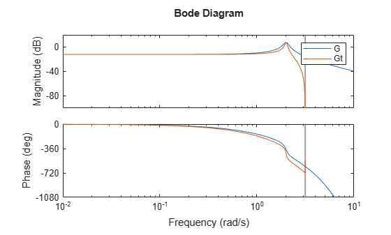
There is a phase lag between the discretized system Gt and the continuous-time system G, which grows as the frequency approaches the Nyquist frequency. This phase lag is largely due to the rounding of the fractional time delay. In this example, the fractional time delay is half the sample time.
Discretize G again using a third-order discrete-time all-pass filter (Thiran filter) to approximate the half-period portion of the delay.
discopts.ThiranOrder = 3;
Gtf = c2d(G,1,discopts);
The ThiranOrder option specifies the order of the Thiran filter that approximates the fractional portion of the delay. The other options in discopts are unchanged. Thus Gtf is a Tustin discretization of G with prewarp at 2 rad/s.
Compare Gtf to G and Gt.
bp = bodeplot(G,Gt,Gtf);
bp.YLimits = {[-100,20];[-1080,0]};
bp.PhaseMatchingEnabled = 'on';
legend('G','Gt','Gtf','Location','SouthWest');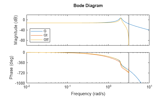
The magnitudes of Gt and Gtf are identical. However, the phase of Gtf provides a better match to the phase of the continuous-time system through the resonance. As the frequency approaches the Nyquist frequency, this phase match deteriorates. A higher-order approximation of the fractional delay would improve the phase matching closer to the Nyquist frequencies. However, each additional order of approximation adds an additional order (or state) to the discretized system.
If your application requires accurate frequency-matching near the Nyquist frequency, use c2dOptions to make c2d approximate the fractional portion of the time delay as a Thiran filter.
See Also
Functions
c2d|c2dOptions|thiran