impulse

R2026b

Impulse response plot of dynamic system; impulse response data

Syntax

[y,tOut] = impulse(sys)

[y,tOut] = impulse(sys,t)

[y,tOut] = impulse(sys,t,p)

[y,t,x] = impulse(___)

[y,t,x,ysd] = impulse(___)

[y,tOut,x,~,pOut] = impulse(sys,t,p)

[___] = impulse(___,Name=Value)

impulse(___)

Description

[y,tOut] = impulse(sys) computes impulse response y of dynamic system sys. impulse automatically determines the time steps and duration of the simulation based on the system dynamics.

[y,tOut] = impulse(sys,t) simulates the response for the time steps specified by t. To define the time steps, you can specify:

• The final simulation time using a scalar value.

• The initial and final simulation times using a two-element vector. (since R2023b)

• All the time steps using a vector.

[y,tOut] = impulse(sys,t,p) specifies the parameter trajectory p for linear parameter-varying (LPV) models. (since R2023a)

[y,t,x] = impulse(___) also returns the state trajectories x, when sys is a state-space model.

[y,t,x,ysd] = impulse(___) returns the standard deviation of the impulse response for identified models. This syntax requires System Identification Toolbox™ software.

[y,tOut,x,~,pOut] = impulse(sys,t,p) returns the parameter trajectories for LPV models. (since R2023a)

[___] = impulse(___,Name=Value) specifies response properties using one or more name-value arguments. For example, impulse(sys,Bias=2) sets the input bias to 2. (since R2026b)

The following name-value arguments override values specified in other input arguments.

• Time — Overrides time values specified using t

• Parameter — Overrides parameter values specified using p

impulse(___) plots the impulse response of sys with default plotting options for all of the previous input argument combinations. For more plot customization options, use impulseplot.

• To plot responses for multiple dynamic systems on the same plot, you can specify sys as a comma-separated list of models. For example, impulse(sys1,sys2,sys3) plots the responses for three models on the same plot.

• To specify a color, line style, and marker for each system in the plot, specify a LineSpec value for each system. For example, impulse(sys1,LineSpec1,sys2,LineSpec2) plots two models and specifies their plot style. For more information on specifying a LineSpec value, see impulseplot.

Examples

Impulse Response of Dynamic System

Plot the impulse response of a continuous-time system represented by the following transfer function.

$$\text{sys}\left(s\right)=\frac{4}{s^2+2s+10}$$

For this example, create a tf model that represents the transfer function. You can similarly plot the impulse response of other dynamic system model types, such as zero-pole gain (zpk) or state-space (ss) models.

sys = tf(4,[1 2 10]);

Plot the impulse response.

impulse(sys)

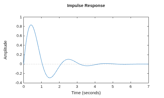
The impulse plot automatically includes a dotted horizontal line indicating the steady-state response. In a MATLAB® figure window, you can right-click the plot to view other impulse-response characteristics such as peak response and transient time.

Impulse Response of Discrete-Time System

Plot the impulse response of a discrete-time system. The system has a sample time of 0.2 s and is represented by the following state-space matrices.

A = [1.6 -0.7;
      1  0];
B = [0.5; 0];
C = [0.1 0.1];
D = 0;

Create the state-space model and plot its impulse response.

sys = ss(A,B,C,D,0.2);
impulse(sys)

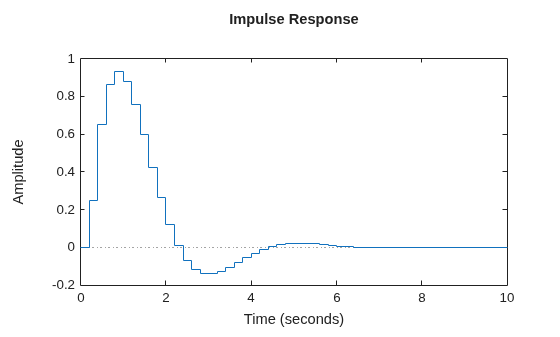
The impulse response reflects the discretization of the model, as it shows the response as computed every 0.2 seconds.

Impulse Response at Specified Times

Examine the impulse response of the following zero-pole-gain model.

sys = zpk(-1,[-0.2+3j,-0.2-3j],1) * tf([1 1],[1 0.05]) 

sys = 
            (s+1)^2
  ----------------------------
  (s+0.05) (s^2 + 0.4s + 9.04)
 
Continuous-time zero/pole/gain model.
Model Properties

impulse(sys)

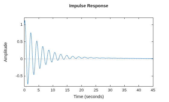
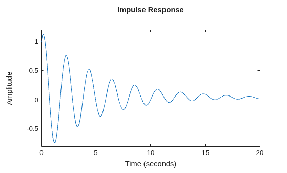
By default, impulse chooses an end time that shows the steady state that the response is trending toward. To get a closer look at the transient response, limit the impulse plot to t = 20 s.

impulse(sys,20)

Alternatively, you can specify the exact times at which you want to examine the impulse response, provided they are separated by a constant interval. For instance, examine the response from the end of the transient until the system reaches steady state.

t = 20:0.2:120;
impulse(sys,t)

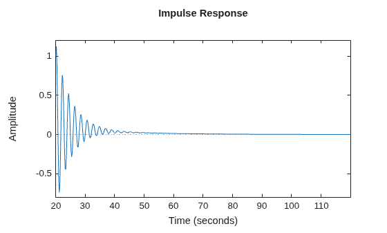
Even though this plot begins at t = 20, impulse always applies the impulse input at t = 0.

Impulse Response Plot of MIMO Systems

Consider the following second-order state-space model:

$$\begin{array}{l}\left[\begin{array}{c}{\underset{}{\overset{\dot{}}{x}}}_1\\ {\underset{}{\overset{\dot{}}{x}}}_2\end{array}\right]=\left[\begin{array}{cc}-0.5572& -0.7814\\ 0.7814& 0\end{array}\right]\left[\begin{array}{c}{x}_1\\ x_2\end{array}\right]+\left[\begin{array}{cc}1& -1\\ 0& 2\end{array}\right]\left[\begin{array}{c}{u}_1\\ u_2\end{array}\right]\\ y=\left[\begin{array}{cc}1.9691& 6.4493\end{array}\right]\left[\begin{array}{c}{x}_1\\ x_2\end{array}\right]\end{array}$$

A = [-0.5572,-0.7814;0.7814,0];
B = [1,-1;0,2];
C = [1.9691,6.4493];
sys = ss(A,B,C,0);

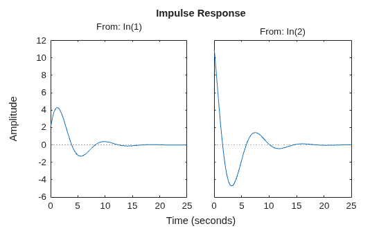
This model has two inputs and one output, so it has two channels: from the first input to the output and from the second input to the output. Each channel has its own impulse response.

When you use impulse, it computes the responses of all channels.

impulse(sys)

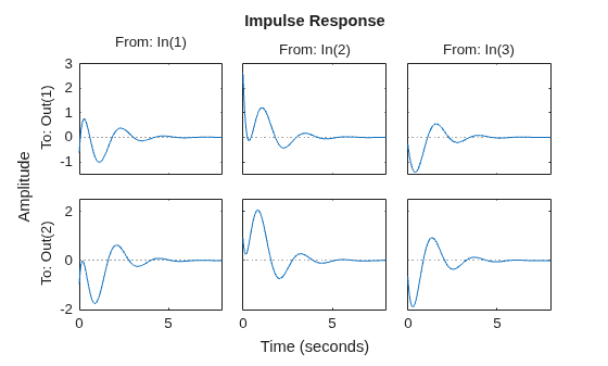
The left plot shows the impulse response of the first input channel, and the right plot shows the impulse response of the second input channel. Whenever you use impulse to plot the responses of a MIMO model, it generates an array of plots representing all the I/O channels of the model. For instance, create a random state-space model with five states, three inputs, and two outputs, and plot its impulse response.

sys = rss(5,2,3);
impulse(sys)

In a MATLAB figure window, you can restrict the plot to a subset of channels by right-clicking on the plot and selecting I/O Selector.

Compare Impulse Response of Multiple Systems

impulse allows you to plot the responses of multiple dynamic systems on the same axis. For instance, compare the closed-loop response of a system with a PI controller and a PID controller. Create a transfer function of the system and tune the controllers.

H = tf(4,[1 2 10]);
C1 = pidtune(H,'PI');
C2 = pidtune(H,'PID');

Form the closed-loop systems and plot their impulse responses.

sys1 = feedback(H*C1,1);
sys2 = feedback(H*C2,1);
impulse(sys1,sys2)
legend('PI','PID','Location','SouthEast')

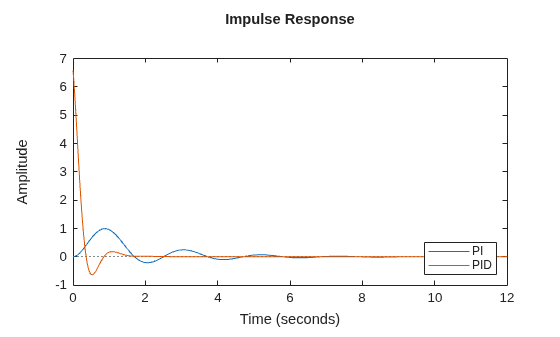
By default, impulse chooses distinct colors for each system that you plot. You can specify colors and line styles using the LineSpec input argument.

 impulse(sys1,'r--',sys2,'b')
 legend('PI','PID','Location','SouthEast')

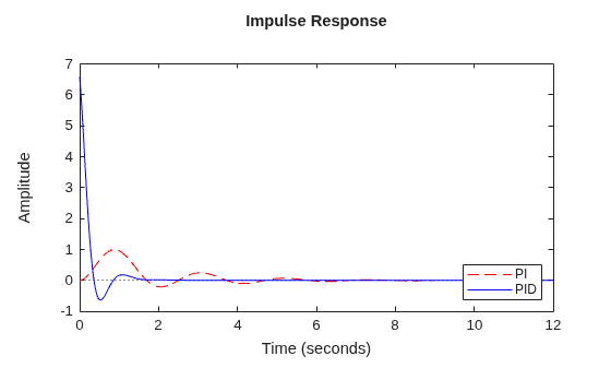
The first LineSpec 'r--' specifies a dashed red line for the response with the PI controller. The second LineSpec 'b' specifies a solid blue line for the response with the PID controller. The legend reflects the specified colors and linestyles. For more plot customization options, use impulseplot.

Impulse Response of Systems in a Model Array

The example Compare Impulse Response of Multiple Systems shows how to plot responses of several individual systems on a single axis. When you have multiple dynamic systems arranged in a model array, impulse plots all their responses at once.

Create a model array. For this example, use a one-dimensional array of second-order transfer functions having different natural frequencies. First, preallocate memory for the model array. The following command creates a 1-by-5 row of zero-gain SISO transfer functions. The first two dimensions represent the model outputs and inputs. The remaining dimensions are the array dimensions.

 sys = tf(zeros(1,1,1,5));

Populate the array.

w0 = 1.5:1:5.5;    % natural frequencies
zeta = 0.5;        % damping constant
for i = 1:length(w0)
   sys(:,:,1,i) = tf(w0(i)^2,[1 2*zeta*w0(i) w0(i)^2]);
end

(For more information about model arrays and how to create them, see Model Arrays.) Plot the impulse responses of all models in the array.

impulse(sys)

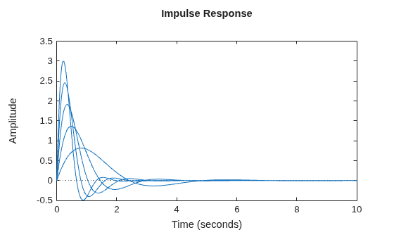
impulse uses the same linestyle for the responses of all entries in the array. One way to distinguish among entries is to use the SamplingGrid property of dynamic system models to associate each entry in the array with the corresponding w0 value.

sys.SamplingGrid = struct('frequency',w0);

Now, when you plot the responses in a MATLAB figure window, you can click a trace to see which frequency value it corresponds to.

Impulse Response Data

When you give it an output argument, impulse returns an array of response data. For a SISO system, the response data is returned as a column vector of length equal to the number of time points at which the response is sampled. You can provide the vector t of time points, or allow impulse to select time points for you based on system dynamics. For instance, extract the impulse response of a SISO system at 101 time points between t = 0 and t = 5 s.

sys = tf(4,[1 2 10]);
t = 0:0.05:5;
y = impulse(sys,t);
size(y)

ans = 1×2

   101     1

For a MIMO system, the response data is returned in an array of dimensions N-by-Ny-by-Nu, where Ny and Nu are the number of outputs and inputs of the dynamic system. For instance, consider the following state-space model, representing a two-input, one-output system.

A = [-0.5572,-0.7814;0.7814,0];
B = [1,-1;0,2];
C = [1.9691,6.4493];
sys = ss(A,B,C,0);

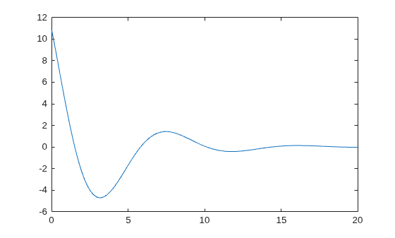
Extract the impulse response of this system at 200 time points between t = 0 and t = 20 s.

t = linspace(0,20,200);
y = impulse(sys,t);
size(y)

ans = 1×3

   200     1     2

y(:,i,j) is a column vector containing the impulse response from the jth input to the ith output at the times t. For instance, extract the impulse response from the second input to the output.

y12 = y(:,1,2);
plot(t,y12)

Impulse Responses of Identified Models with Confidence Regions

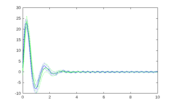
Compare the impulse response of a parametric identified model to a non-parametric (empirical) model. Also view their 3 $$\sigma$$ confidence regions.

Load the data.

load iddata1 z1

Estimate a parametric model.

sys1 = ssest(z1,4);

Estimate a non-parametric model.

sys2 = impulseest(z1);

Plot the impulse responses for comparison.

t = (0:0.1:10)';
[y1, ~, ~, ysd1] = impulse(sys1,t);
[y2, ~, ~, ysd2] = impulse(sys2,t);
plot(t, y1, 'b', t, y1+3*ysd1, 'b:', t, y1-3*ysd1, 'b:')
hold on
plot(t, y2, 'g', t, y2+3*ysd2, 'g:', t, y2-3*ysd2, 'g:')

Impulse Response of Identified Time-Series Model

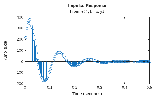
Compute the impulse response of an identified time-series model.

A time-series model, also called a signal model, is one without measured input signals. The impulse plot of this model uses its (unmeasured) noise channel as the input channel to which the impulse signal is applied.

Load the data.

load iddata9;

Estimate a time-series model.

sys = ar(z9, 4);

sys is a model of the form A y(t) = e(t), where e(t) represents the noise channel. For computation of impulse response, e(t) is treated as an input channel, and is named e@y1.

Plot the impulse response.

impulse(sys)

Configure Options for Impulse Response

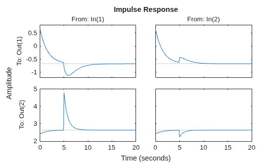
Create a state-space model.

A = [-0.8429,-0.2134;-0.5162,-1.2139];
B = [0.7254,0.7147;0,-0.2050];
C = [-0.1241,1.4090;1.4897,1.4172];
D = [0.6715,0.7172;-1.2075,0];
sys = ss(A,B,C,D);

Compute the impulse response, specifying response options using name-value arguments.

t = 0:0.1:20;
impulse(sys,t, ...
    Bias=[-2,3], ...
    Amplitude=[2,-0.5], ...
    InitialCondition=[0.1,-0.1], ...
    Delay=5)

Impulse Response of LPV Model

This example shows how to simulate the impulse response of an LPV model. This example simulates the closed-loop response of a levitating ball model defined in fcnMaglev.m to a disturbance $\text{du}$.

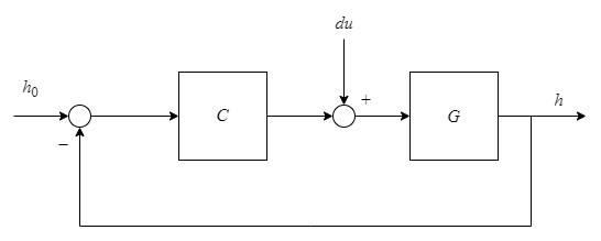
You must set the reference to $h_0$ to properly initialize the system and maintain it around $h$ = $h_0$.

Create the model and discretize it.

hmin = 0.05; 
hmax = 0.25;
h0 = (hmin+hmax)/2;
Ts = 0.01;
Glpv = lpvss("h",@fcnMaglev,0,0,h0);
Glpvd = c2d(Glpv,Ts,"tustin"); 

Sample the LPV model for three height values and tune a PID controller.

hpid = linspace(hmin,hmax,3);
[Ga,Goffset] = sample(Glpvd,[],hpid);
wc = 50;
Ka = pidtune(Ga,"pidf",wc);
Ka.Tf = 0.01;

Create the gain-scheduled PID controller.

Ka.SamplingGrid = struct("h",hpid);
Koffset = struct("y",{Goffset.u});
Clpv = ssInterpolant(ss(Ka),Koffset);

Create the closed-loop model.

CL = feedback(Glpvd*[1,Clpv],1,2,1);
CL.InputName = {'du';'href'};
CL.OutputName = "h";

Get steady-state current for $h$ = $h_0$ to size the disturbance.

[~,~,~,~,~,~,~,u0] = Glpv.DataFunction(0,h0);

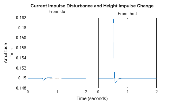
Response to impulse change in $\text{du}$ and $h_0$.

t = 0:Ts:2;
pFcn = @(k,x,u) x(1);
IC = findop(CL,t(1),h0,u=[u0;h0]);
impulseplot(CL,t,pFcn, ...
    Amplitude=0.2*[u0;h0]*Ts, ...
    Delay=0.5, ...
    InitialCondition=IC)
title("Current Impulse Disturbance and Height Impulse Change")

Compute Impulse Response of Model with Complex Coefficients

Create a state-space model with complex coefficients.

A = [-2-2i -2;1 0];
B = [2;0];
C = [0 0.5+2.5i];
D = 0;
sys = ss(A,B,C,D);

Compute the impulse response of the system.

[y,t] = impulse(sys);

The resulting response data contains complex output values.

y

Input Arguments

sys — Dynamic system

dynamic system model | model array

Dynamic system, specified as a SISO or MIMO dynamic system model or an array of dynamic system models. You can use these types of dynamic systems:

• Continuous-time or discrete-time numeric LTI models, such as tf, zpk, or ss models.

• Generalized or uncertain LTI models such as genss or uss models. (Using uncertain models requires Robust Control Toolbox™ software.)

  • For tunable control design blocks, the function evaluates the model at its current value for both plotting and returning response data.

  • For uncertain control design blocks, the function plots the nominal value and random samples of the model. When you use output arguments, the function returns response data for the nominal model only.

• Sparse state-space models such as sparss and mechss models.

• Identified LTI models, such as idtf, idss, or idproc models. For such models, the function can also plot confidence intervals and return standard deviations of the frequency response. See Step Responses of Identified Models with Confidence Regions. (Using identified models requires System Identification Toolbox software.)

• Linear time-varying (ltvss) and linear parameter-varying (lpvss) models.

This function does not support frequency-response data models such as frd, genfrd, or idfrd models.

If sys is an array of models, the function plots the responses of all models in the array on the same axes. See Step Response of Systems in a Model Array.

t — Time steps

positive scalar | two-element vector | vector | []

Time steps at which to compute the response, specified as one of these values:

• Positive scalar tFinal— Compute the response from t = 0 to t = tFinal.

• Two-element vector [t0 tFinal] — Compute the response from t = t0 to t = tFinal. (since R2023b)

• Vector Ti:dt:Tf— Compute the response for the time points specified in t.

  • For continuous-time systems, dt is the sample time of a discrete approximation to the continuous system.

  • For discrete-time systems with a specified sample time, dt must match the sample time property Ts of sys.

  • For discrete-time systems with an unspecified sample time (Ts = -1), dt must be 1.

• [] — Automatically select time values based on system dynamics.

When you specify a time range using either tFinal or [t0 tFinal]:

• For continuous-time systems, the function automatically determines the size of the time step and number of points based on the system dynamics.

• For discrete-time systems with a specified sample time, the function uses the sample time of sys as the step size.

• For discrete-time systems with unspecified sample time (Ts = -1), the function interprets tFinal as the number of sampling periods to simulate with a sample time of 1 second.

Express t using the time units specified in the TimeUnit property of sys.

Before R2026a: Specify time values using the Responses.SourceData.TimeSpec property.

Before R2026b: This property is called TimeSpec.

p — LPV model parameter trajectory

matrix | function handle

Parameter trajectory of the LPV model, specified as a matrix or a function handle.

• For exogenous or explicit trajectories, specify p as a matrix with dimensions N-by-Np, where N is the number of time samples and Np is the number of parameters.

  Thus, the row vector p(i,:) contains the parameter values at the ith time step.

• For endogenous or implicit trajectories, specify p as a function handle of the form p = F(k,x,u) that gives parameters as a function of time sample k, state x, and input u. impulse only supports this option for discrete-time LPV models.

  This option is useful when you want to simulate quasi-LPV models.

Name-Value Arguments

Specify optional pairs of arguments as Name1=Value1,...,NameN=ValueN, where Name is the argument name and Value is the corresponding value. Name-value arguments must appear after other arguments, but the order of the pairs does not matter.

Example: impulse(sys,Bias=2) sets the input bias to 2.

Time — Time values

scalar | vector | []

Since R2026b

Time steps at which to compute the response, specified as one of these values. Specifying time values using a name-value argument overrides the time values that you specify using t.

• Positive scalar tFinal— Compute the response from t = 0 to t = tFinal.

• Two-element vector [t0 tFinal] — Compute the response from t = t0 to t = tFinal.

• Vector Ti:dt:Tf— Compute the response for the time points specified in t.

  • For continuous-time systems, dt is the sample time of a discrete approximation to the continuous system.

  • For discrete-time systems with a specified sample time, dt must match the sample time property Ts of sys.

  • For discrete-time systems with an unspecified sample time (Ts = -1), dt must be 1.

• [] — Automatically select time values based on system dynamics.

When you specify a time range using either tFinal or [t0 tFinal]:

• For continuous-time systems, the function automatically determines the size of the time step and number of points based on the system dynamics.

• For discrete-time systems with a specified sample time, the function uses the sample time of sys as the step size.

• For discrete-time systems with unspecified sample time (Ts = -1), the function interprets tFinal as the number of sampling periods to simulate with a sample time of 1 second.

Express Time using the time units specified in the TimeUnit property of sys.

Parameter — LPV model parameter trajectory

matrix | function handle

Since R2026b

LPV model parameter trajectory, specified as a matrix or a function handle. Specifying parameter values using a name-value argument overrides the parameter values that you specify using p.

• For exogenous or explicit trajectories, specify Parameter as a matrix with dimensions N-by-Np, where N is the number of time samples and Np is the number of parameters.

  Thus, the row vector p(i,:) contains the parameter values at the ith time step.

• For endogenous or implicit trajectories, specify Parameter as a function handle of the form p = F(t,x,u) in continuous time and p = F(k,x,u) in discrete time that gives parameters as a function of time t or time sample k, state x, and input u. For implicit trajectories, you must specify an initial condition for the simulation.

  This option is useful when you want to simulate quasi-LPV models.

Amplitude — Input level change

1 (default) | scalar | vector

Since R2026b

Input level change relative to the input signal bias, specified as a scalar or vector.

• For single-input systems, Amplitude is a scalar value.

• For multi-input systems, Amplitude is a vector of length N _u, where N _u is the number of input channels. Each vector value corresponds to the level change amplitude in that input channel. The functions compute the responses one input channel at a time.

Complex Number Support: Yes

Bias — Baseline input signal value

0 (default) | scalar | vector | "u0"

Since R2026b

Baseline input signal value, specified as a scalar or vector.

• For single-input systems, Bias is a scalar value.

• For multi-input systems, Bias is a vector of length N _u, where N _u is the number of input channels. Each vector value corresponds to the signal value in that input channel. The functions compute the responses one input channel at a time.

• For state-space models with offsets, set Bias = "u0" to apply the step or impulse change relative to the model offsets u ₀, u ₀(t) of the LTV model, or u ₀(t,p) of the LPV model. For LTV and LPV models, this is the u0 output of the data function. The total input signal is then u ₀ + u(t).

Delay — Input signal delay

0 (default) | nonnegative scalar

Since R2026b

Input signal delay, specified as a nonnegative scalar value. This value specifies when the change occurs relative to the simulation start time T ₀.

InitialCondition — Initial condition

[] (default) | vector | "x0" | operating condition created using findop | initialCondition object

Since R2026b

Initial condition, specified as one of these values:

• [] — Start simulation from the steady-state condition for the input value specified in Bias. For state-space models without internal delays, the initial state x_init is the solution to the following, where U is the Bias value:

  • Continuous time — 0 = A x_init + B U

  • Discrete time — x_init = A x_init + B U

• Vector of initial state values with length equal to the number of states in the model — Start simulation from the specified initial state and use Bias as the initial input value.

• "x0" — Use Bias as the initial input value and evaluate state offset value x ₀ for state-space models, x ₀(T ₀) for LTV models, or x ₀(T ₀,p(T ₀)) for LPV models. For LTV and LPV models, the state offset value is the x0 output of the data function evaluated at t = T ₀.

• initialCondition (System Identification Toolbox) object for identified models (requires System Identification Toolbox software) — Start simulation from the specified initial state and use Bias as the initial input value.

• Operating condition created using findop — An operating point object allows you to start the simulation from a steady-state operating condition with nonzero past u, w, and y values. When you specify an operating point object, the value of Bias is ignored.

Output Arguments

y — Impulse response data

array

Impulse response data, returned as an array.

• For SISO systems, y is a column vector of the same length as t (if provided) or tOut (if you do not provide t).

• For single-input, multi-output systems, y is a matrix with as many rows as time samples and as many columns as outputs. Thus, the jth column of y, or y(:,j), contains the impulse response of from the input to the jth output.

• For MIMO systems, the impulse responses of each input channel are stacked up along the third dimension of y. The dimensions of y are then N-by-Ny-by-Nu, where:

  • N is the number of time samples.

  • Ny is the number of system outputs.

  • Nu is the number of system inputs.

  Thus, y(:,i,j) is a column vector containing the impulse response from the jth input to the ith output at the times specified in t or tOut.

• For systems with complex coefficients, y is an array of complex values. (since R2025a)

tOut — Times at which impulse response is computed

vector

Times at which impulse response is computed, returned as a vector. When you do not provide a specific vector t of times, impulse chooses this time vector based on the system dynamics. The times are expressed in the time units of sys.

x — State trajectories

array

State trajectories, returned as an array. When sys is a state-space model, x contains the evolution of the states of sys at each time in t or tOut. The dimensions of x are N-by-Nx-by-Nu, where:

• N is the number of time samples.

• Nx is the number of states.

• Nu is the number of system inputs.

Thus, the evolution of the states in response to an impulse injected at the kth input is given by the array x(:,:,k). The row vector x(i,:,k) contains the state values at the ith time step.

For systems with complex coefficients, x is an array of complex values. (since R2025a)

ysd — Standard deviation of impulse response

array

Standard deviation of the impulse response of an identified model, returned as an array of the same dimensions as y. If sys does not contain parameter covariance information, then ysd is empty.

pOut — Parameter trajectories

array

Parameter trajectories, returned as an array. When sys is a linear-parameter varying model, pOut contains the evolution of the parameters of sys at each time in t or tOut. The dimensions of pOut are N-by-Np-by-Nu, where:

• N is the number of time samples.

• Np is the number of parameters.

• Nu is the number of system inputs.

Thus, the evolution of the parameters in response to a signal injected at the kth input is given by the array pOut(:,:,k). The row vector pOut(i,:,k) contains the parameter values at the ith time step.

Limitations

• The impulse response of a continuous system with nonzero D matrix is infinite at t = 0. impulse ignores this discontinuity and returns the lower continuity value Cb at t = 0.

• The impulse command does not work on continuous-time models with internal delays. For such models, use pade to approximate the time delay before computing the impulse response.

• The impulse command does not support simulation along an implicit parameter trajectory for continuous-time LPV models.

Tips

• To simulate system responses to arbitrary input signals, use lsim.

• When you need additional plot customization options, use impulseplot instead.

• Plots created using impulse do not support multiline titles or labels specified as string arrays or cell arrays of character vectors. To specify multiline titles and labels, use a single string with a newline character.

  impulse(sys)
  title("first line" + newline + "second line");

Algorithms

Continuous-time LTI models are first converted to state-space form. The impulse response of a single-input state-space model

$$\begin{array}{l}\dot{x}=Ax+bu\\ y=Cx\end{array}$$

is equivalent to the following unforced response with initial state b.

$$\begin{array}{cc}\dot{x}=Ax,& x(0)=b\\ y=Cx& \end{array}$$

To simulate this response, the system is discretized using zero-order hold on the inputs. The sample time is chosen automatically based on the system dynamics, except when a time vector t = T0:dt:Tf is supplied. Hence, dt is used as sample time.

Version History

Introduced before R2006a

R2026b: Specify response options using name-value arguments

You can now specify response options using these name-value arguments:

• Time — Time values

• Bias — Baseline input signal value

• Amplitude — Input level change

• Delay — Input signal delay

• InitialCondition — System initial condition

• Parameter — LPV model parameter trajectory

These options replace response configuration using a RespConfig object. For more information, see Setting response options using RespConfig object not recommended.

R2026b: Setting response options using RespConfig object not recommended

Setting response options using a RespConfig object is not recommended. Use the Bias, Amplitude, Delay, and InitialCondition name-value arguments instead.

This table shows some uses of RespConfig and how to update your code to use the new name-value arguments. Here, sysLPV is a linear parameter-varying model.

Not Recommended	Recommended
config = RespConfig( ... Amplitude=0.5, ... Bias=1, ... Delay=2, ... InitialState=[1 2 3]); [y,t] = impulse(sys,config)	[y,t] = impulse(sys, ... Amplitude=0.5, ... Bias=1, ... Delay=2, ... InitialCondition=[1 2 3])
config = RespConfig( ... Bias=-1, ... InitialParameter=pinit); [y,t] = impulse(sysLPV,t,pFcn,config)	IC = findop(sysLPV,t(1),pinit,u=-1); [y,t] = impulse(sysLPV,t,pFcn,InitialCondition=IC)
For LPV systems with state offsets: config = RespConfig( ... InitialState="x0", ... InitialParameter=pinit) [y,t] = impulse(sysLPV,t,pFcn,config)	[~,~,~,~,~,~,x0] = sysLPV.DataFunction(t(1),pinit); [y,t] = impulse(sysLPV,t,pFcn,InitialCondition=x0)
For LPV systems with input offsets: config = RespConfig( ... Bias="u0", ... InitialParameter=pinit) [y,t] = impulse(sysLPV,t,pFcn,config)	[~,~,~,~,~,~,~,u0] = sysLPV.DataFunction(t(1),pinit); IC = findop(sysLPV,tinit,pinit,u=u0); [y,t] = impulse(sysLPV,t,pFcn,InitialCondition=IC)

R2026a: Support for sparse index-2 models

Starting in R2026a, the impulse function supports sparse index-2 DAEs.

R2025a: Support for dynamic systems with complex coefficients

Starting in R2025a, the impulse function supports dynamic systems with complex coefficients.

R2024b: gca now returns chart object

For plots created using impulse, the gca function now returns an impulseplot chart object rather than an axes within the plot.

R2023b: Response characteristics computation changes

The computation of some response characteristics has changed when using a nondefault configuration created using RespConfig.

• The Peak Response characteristic now shows the maximum deviation from the initial output value. That is, the peak value of |y(t) – y_init| when t ≥ t₀ + t_d, where y_init is the output value just before the impulse.

  As a result, in the Peak Response data tip, Peak amplitude is renamed to Peak deviation.

• Settling time and transient time are now computed relative to the time when the impulse occurs (t = t₀ + t_d). This ensures that these characteristics are unaffected by the delay.

In general, the software computes the response characteristics from the time of the impulse, with the initial output value y_init as the value just before the impulse.

R2023b: New syntax

Use the new syntax [y,tOut] = impulse(sys,[t0,tFinal]) to compute the impulse response from time t0 to tFinal. For configurations with a delay td, the function applies the impulse at time t = t0 + td.

R2023a: Support for nonzero start time

You can now specify a nonzero start time for the impulse command using a time vector input of the form Ti:dt:Tf. Previously, the command always applied the input at t = 0, regardless of Ti.