Compare Residual Recurrent Neural Network Structures for Digital Predistortion Design
This example shows how to design, train, test, and compare several residual recurrent neural network (RNN) structures to apply digital predistortion (DPD). DPD offsets the effects of nonlinearities in a power amplifier (PA). In this example, you:
Design and train LSTM, BiLSTM, GRU, BiGRU, and their residual versions as a DPD.
Perform hyperparameter optimization and comparison using the Experiment Manager.
Test the DPD structures using a real PA.
Compare the results to that of multi-layer perceptron (MLP) and cross-term memory polynomial DPD.
Introduction
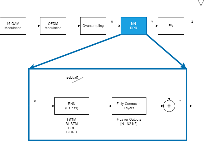
This example focuses on offline training of the RNN-based DPD (RNN-DPD). For details on offline training using an MLP, see the Neural Network for Digital Predistortion Design-Offline Training example. The RNN-DPD consists of L units of RNN followed by three fully connected layers with N1, N2, and N3 output neurons. To test the effect of residual training, add a bypass path. Split the complex input, u, into a 2-by-1 array of in-phase and quadrature components and combine the 2-by-1 output of the NN into a complex number, y.

L  = 50;    % Number of RNN units
N1 = 100;   % Number of outputs of 1st fully connected layer
N2 = 50;    % Number of outputs of 2nd fully connected layer
N3 = 2;     % Number of outputs of 3rd fully connected layer
RNN Structures
Design and train four different RNN structures together with their residual counterparts as shown in [1].
LSTM
A long short-term memory (LSTM) neural network can learn long-term dependencies between time steps of sequence data. The core components of an LSTM neural network are a sequence input layer and an LSTM layer. A sequence input layer inputs sequence or time series data into the neural network. An LSTM layer learns long-term dependencies between time steps of sequence data. For more information, see Long Short-Term Memory Neural Networks (Deep Learning Toolbox).
layers = [...
  sequenceInputLayer(2,Name="input",MinLength=1)

  lstmLayer(L,Name="lstm",OutputMode="sequence")

  fullyConnectedLayer(N1,Name="linear1")
  leakyReluLayer(0.01,Name="leakyRelu1")

  fullyConnectedLayer(N2,Name="linear2")
  leakyReluLayer(0.01,Name="leakyRelu2")

  fullyConnectedLayer(N3,Name="linearOutput")
  ];
netLSTM = dlnetwork(layers,Initialize=false);
BiLSTM
A bidirectional LSTM (BiLSTM) operation learns bidirectional long-term dependencies between time steps of time series or sequence data. These dependencies are useful when you want the network to learn from the complete time series at each time step. This network introduces a delay equal to the number of samples in the input sequence. For more information, see the bilstmLayer (Deep Learning Toolbox) function.
layers = [...
  sequenceInputLayer(2,Name="input",MinLength=1)

  bilstmLayer(L,Name="bilstm",OutputMode="sequence")

  fullyConnectedLayer(N1,Name="linear1")
  leakyReluLayer(0.01,Name="leakyRelu1")

  fullyConnectedLayer(N2,Name="linear2")
  leakyReluLayer(0.01,Name="leakyRelu2")

  fullyConnectedLayer(N3,Name="linearOutput")
  ];
netBiLSTM = dlnetwork(layers,Initialize=false);
GRU
The gated recurrent unit (GRU) layer allows a network to learn dependencies between time steps in time series and sequence data. The GRU solves the vanishing gradient problem of standard RNNs by using two gates. The update gate determines how much of the past information needs to be passed along to the future and the reset gate decides how much of the past information to forget. For more information, see the gruLayer (Deep Learning Toolbox) function.
layers = [...
  sequenceInputLayer(2,Name="input",MinLength=1)

  gruLayer(L,Name="gru",OutputMode="sequence")

  fullyConnectedLayer(N1,Name="linear1")
  leakyReluLayer(0.01,Name="leakyRelu1")

  fullyConnectedLayer(N2,Name="linear2")
  leakyReluLayer(0.01,Name="leakyRelu2")

  fullyConnectedLayer(N3,Name="linearOutput")
  ];
netGRU = dlnetwork(layers,Initialize=false);
BiGRU
The bidirectional GRU (BiGRU) layer extends the GRU model by processing the data in both forward and backward directions, similar to BiLSTM. This approach allows the model to capture information from both past (backward) and future (forward) states. Implement a BiGRU layer using helperFlipLayer and gruLayer functions.
net = dlnetwork;
net = addLayers(net,sequenceInputLayer(2,Name="input",MinLength=1));
net = addLayers(net,gruLayer(L,Name="gru1",OutputMode="sequence"));
layers = [helperFlipLayer("flip1")
  gruLayer(L,Name="gru2",OutputMode="sequence")
  helperFlipLayer("flip2")];
net = addLayers(net,layers);

layers = [concatenationLayer(1, 2, Name="cat")

fullyConnectedLayer(N1,Name="linear1")
leakyReluLayer(0.01,Name="leakyRelu1")

fullyConnectedLayer(N2,Name="linear2")
leakyReluLayer(0.01,Name="leakyRelu2")

fullyConnectedLayer(N3,Name="linearOutput")
];

net = addLayers(net,layers);

net = connectLayers(net, "input", "gru1");
net = connectLayers(net, "gru1", "cat/in1");
net = connectLayers(net, "input", "flip1");
netBiGRU = connectLayers(net, "flip2", "cat/in2");
Prepare Data
Generate training, validation, and testing data. Use the training and validation data to train the RNN-DPD. Use the test data to evaluate the RNN-DPD performance. For details, see the Data Preparation for Neural Network Digital Predistortion Design example.
Choose Data Source
Choose the data source for the system. This example uses an NXP™ Airfast LDMOS Doherty PA, which is connected to a local NI™ VST, as described in the Power Amplifier Characterization example. If you do not have access to a PA, run the example with the simulated PA or saved data. The simulated PA uses a neural network PA model, which is trained using data captured from the PA using an NI VST. The example downloads data files including the results of the Example Manager runs. The saved data option uses a lookup table and not all input signals have a saved output signal.
dataSource ="Simulated PA"; helperNNDPDDownloadData("rnn")
Starting download of data files from:
	https://www.mathworks.com/supportfiles/spc/NNDPD/rnn_dpd.zip
Download complete. Extracting files.
Extract complete.
Generate Training Data
Generate oversampled OFDM signals.
[txWaveTrain,txWaveVal,txWaveTest,qamRefSymTrain,qamRefSymVal, ...
  qamRefSymTest,ofdmParams] = generateOversampledOFDMSignals;
Fs = ofdmParams.SampleRate;
Pass signals through the PA using the helperNNDPDPowerAmplifier System object™.
pa = helperNNDPDPowerAmplifier(DataSource=dataSource,SampleRate=Fs);
paOutputTrain = pa(txWaveTrain);
paOutputVal = pa(txWaveVal);
Preprocess the data to generate input vectors containing IQ samples. Create subsequences using a sliding window of length sequenceLength. Move the window stepSize samples to create the next subsequence. Each subsequence is a training sample. Use 1/3 the number of training samples for validation.
normFactor = std(txWaveTest); sequenceLength =300; stepSize =
100; dataLength = size(txWaveTrain,1); numSeq = floor((dataLength-sequenceLength)/stepSize); inputCellTrain = cell(numSeq,1); outputCellTrain = cell(numSeq,1); dataCnt = 1; for p=1:stepSize:dataLength-sequenceLength inputCellTrain{dataCnt} = [real(paOutputTrain(p:sequenceLength+p-1,1)) ... imag(paOutputTrain(p:sequenceLength+p-1,1))]/normFactor; outputCellTrain{dataCnt} = [real(txWaveTrain(p:sequenceLength+p-1,1)) ... imag(txWaveTrain(p:sequenceLength+p-1,1))]/normFactor; dataCnt = dataCnt+1; end dataLength = size(txWaveVal,1) / 3; numSeq = floor((dataLength-sequenceLength)/stepSize); inputCellVal = cell(numSeq,1); outputCellVal = cell(numSeq,1); dataCnt = 1; for p=1:stepSize:dataLength-sequenceLength inputCellVal{dataCnt} = [real(paOutputVal(p:sequenceLength+p-1,1)) ... imag(paOutputVal(p:sequenceLength+p-1,1))]/normFactor; outputCellVal{dataCnt} = [real(txWaveVal(p:sequenceLength+p-1,1)) ... imag(txWaveVal(p:sequenceLength+p-1,1))]/normFactor; dataCnt = dataCnt+1; end
Compare Networks and Optimize Hyperparameters
This example optimizes the hyperparameters L and N1 while comparing the RNN structures. Use Experiment Manager to train and obtain validation loss and RMSE values in parallel.
Configure Experiment Manager
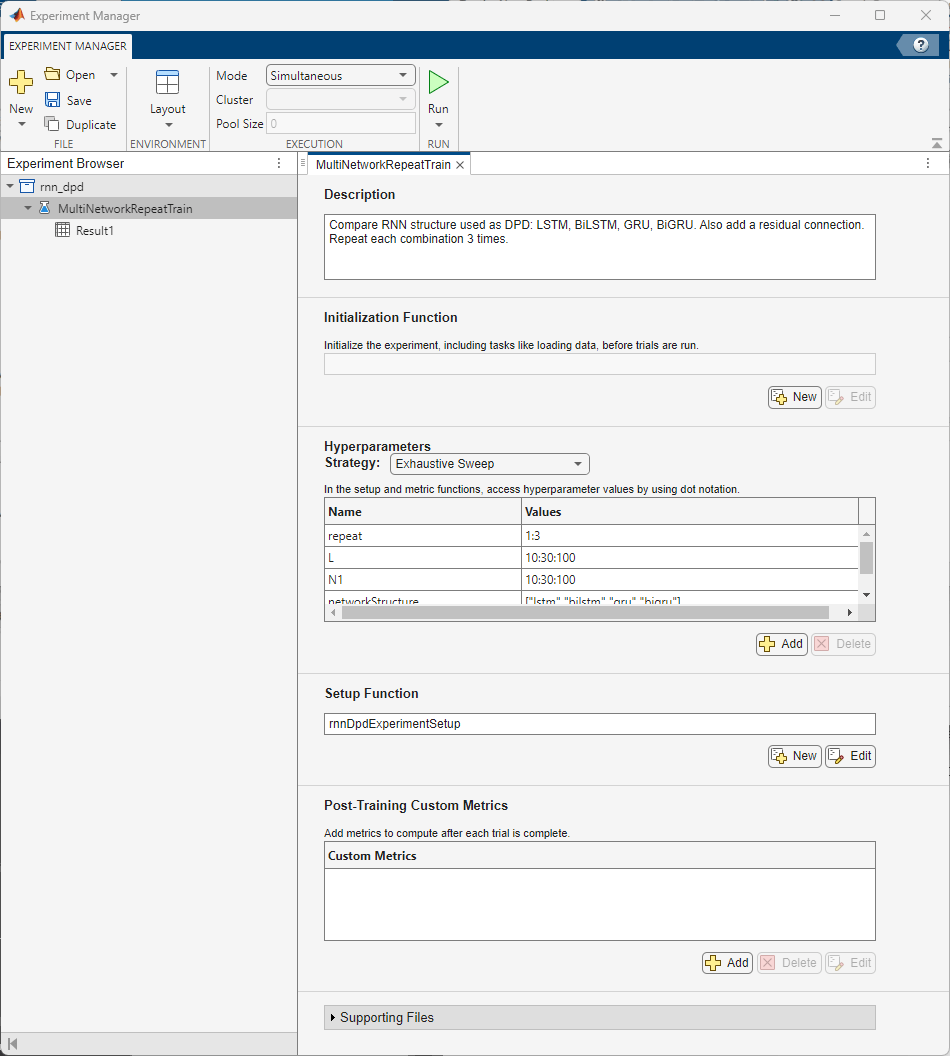
Configure Experiment Manager to sweep over the hyperparameters for the eight RNN structures: LSTM, Residual LSTM, BiLSTM, Residual BiLSTM, GRU, Residual GRU, BiGRU, Residual BiGRU. To reduce the number of hyperparameters, sweep over L and N1, and set N2 as half of N1. Configure the hyperparameters as follows:
Strategy: Exhaustive sweep
L: 10:30:100
N1: 10:30:100
Network structure: LSTM, BiLSTM, GRU, BiGRU
Residual connection active: false, true
The training algorithm initializes the neural network with random weights. As a result, the trained network can converge to a different local minima. Add an extra parameter, repeat, to train the neural network multiple times. Select the best one.
Set Mode to Simultaneous to run the trials in parallel. If you have access to a cluster, you can also run the trials on a cluster and massively parallelize hyperparameter optimization. On a PC with an AMD EPYC 7262 8-core processor, 384 trials with validation patience of 3 and 8 workers, run in about 12 hours.

The rnnDpdExperimentSetup function sets up the network and generates training data. The emACPR, emEVM, emNME functions calculate the metrics.
The rnn_dpd.zip file contains a preconfigured project and results.
exampleDir = pwd;
projectName = "rnn_dpd";
projRoot = fullfile(pwd,projectName);
To open the project, start Experiment Manager and open the following file.
disp(fullfile(".","rnn_dpd","Rnn_dpd.prj"))
.\rnn_dpd\Rnn_dpd.prj
Explore Results
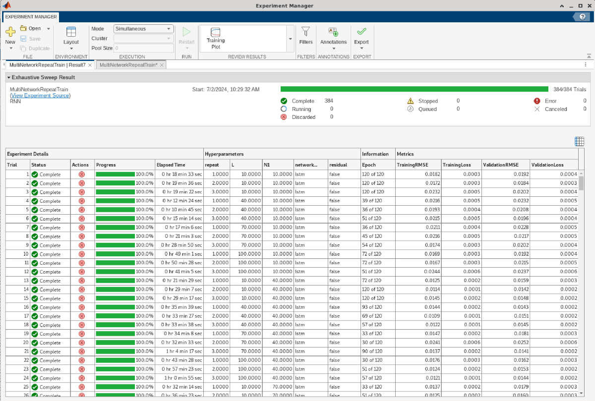
Experiment Manager shows the results of each trial as a table. Export the results table by using the Export > Results Table button.

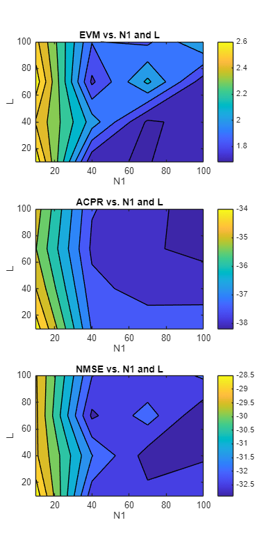
The rnnDPDMultiNetworkRepeatTrainResults.mat file contains the results exported from Results 1 of the MultiNetworkRepeatTrain experiment. Load the results table and plot filled contours to examine the hyperparameter space for EVM, ACPR, and NMSE values. Opening the project changes the current directory. Reset the current directory.
cd(exampleDir)
switch dataSource
  case "Simulated PA"
    load rnnDPDMultiNetworkRepeatTrainResults.mat resultsTable
  case "Saved data"
    load rnnDPDMultiNetworkRepeatSavedDataTrainResults.mat resultsTable
  otherwise
    error("Saved results are not available when data source is %d",dataSource)
end
resultsTable
resultsTable=384×4 table
     1    "Complete"    100    00:18:33    1     10    10    "lstm"    false    3    120    "120 of 120"    26280    "Piecewise"    2.9007e-04    654    3    "Loss"    "Best validation"    "Single CPU"    0.0182    3.3101e-04    0.0192    3.6849e-04
     2    "Complete"    100    00:19:36    2     10    10    "lstm"    false    3    120    "120 of 120"    26280    "Piecewise"    2.9007e-04    654    3    "Loss"    "Best validation"    "Single CPU"    0.0172    2.9449e-04    0.0184    3.3764e-04
     3    "Complete"    100    00:19:22    3     10    10    "lstm"    false    3    120    "120 of 120"    26280    "Piecewise"    2.9007e-04    654    3    "Loss"    "Best validation"    "Single CPU"    0.0232    5.3964e-04    0.0202    4.0619e-04
     4    "Complete"    100    00:12:24    1     40    10    "lstm"    false    3    120     "39 of 120"     8502    "Piecewise"        0.0016    654    3    "Loss"    "Best validation"    "Single CPU"    0.0216    4.6627e-04    0.0232    5.3908e-04
     5    "Complete"    100    00:10:45    2     40    10    "lstm"    false    3    120     "36 of 120"     7848    "Piecewise"        0.0016    654    3    "Loss"    "Best validation"    "Single CPU"    0.0193    3.7324e-04    0.0208    4.3208e-04
     6    "Complete"    100    00:15:14    3     40    10    "lstm"    false    3    120     "51 of 120"    11118    "Piecewise"        0.0011    654    3    "Loss"    "Best validation"    "Single CPU"    0.0215    4.6164e-04    0.0196    3.8491e-04
     7    "Complete"    100    00:17:06    1     70    10    "lstm"    false    3    120     "36 of 120"     7848    "Piecewise"        0.0016    654    3    "Loss"    "Best validation"    "Single CPU"    0.0211    4.4431e-04    0.0228    5.1779e-04
     8    "Complete"    100    00:21:03    2     70    10    "lstm"    false    3    120     "45 of 120"     9810    "Piecewise"        0.0011    654    3    "Loss"    "Best validation"    "Single CPU"    0.0216    4.6606e-04    0.0217    4.7098e-04
     9    "Complete"    100    00:28:50    3     70    10    "lstm"    false    3    120     "54 of 120"    11772    "Piecewise"        0.0011    654    3    "Loss"    "Best validation"    "Single CPU"    0.0174    3.0144e-04    0.0202    4.0890e-04
    10    "Complete"    100    00:49:01    1    100    10    "lstm"    false    3    120     "72 of 120"    15696    "Piecewise"    6.8656e-04    654    3    "Loss"    "Best validation"    "Single CPU"    0.0169    2.8394e-04    0.0192    3.6861e-04
    11    "Complete"    100    00:50:28    2    100    10    "lstm"    false    3    120     "72 of 120"    15696    "Piecewise"    6.8656e-04    654    3    "Loss"    "Best validation"    "Single CPU"    0.0167    2.7807e-04    0.0215    4.6344e-04
    12    "Complete"    100    00:41:05    3    100    10    "lstm"    false    3    120     "51 of 120"    11118    "Piecewise"        0.0011    654    3    "Loss"    "Best validation"    "Single CPU"    0.0244    5.9417e-04    0.0237    5.6107e-04
    13    "Complete"    100    00:21:29    1     10    40    "lstm"    false    3    120     "72 of 120"    15696    "Piecewise"    6.8656e-04    654    3    "Loss"    "Best validation"    "Single CPU"    0.0125    1.5642e-04    0.0159    2.5262e-04
    14    "Complete"    100    00:29:07    2     10    40    "lstm"    false    3    120    "120 of 120"    26280    "Piecewise"    2.9007e-04    654    3    "Loss"    "Best validation"    "Single CPU"    0.0114    1.2978e-04    0.0142    2.0116e-04
      ⋮
Measure EVM, ACPR, and NMSE
The PA might not be available during training. Measure EVM, ACPR, and NMSE metrics after training using the PA. For each trial, the helperExperimentManagerTrial function, returns the inputs and outputs of the trial. The trialOut structure contains the trained RNN. Pass the signals through the RNN and then pass the output of the DPD through the PA. Measure the metrics using the PA output. Append the measurements to the results table.
The processing takes about 20 minutes. To load the saved results, set processNow to false.
processNow =false; if processNow switch dataSource case "Saved data" expDir = fullfile(pwd,"rnn_dpd","Results","MultiNetworkRepeatTrainSavedData_Result2_20240708T130348/"); case "Simulated PA" expDir = fullfile(pwd,"rnn_dpd","Results","MultiNetworkRepeatTrain_Result7_20240702T102933/"); case "NI VST" expDir = selectExperimentResultsFolder(); end numTrials = size(resultsTable,1); resultsTable.Metrics.EVM_percent = zeros(numTrials,1); resultsTable.Metrics.ACPR_dB = zeros(numTrials,1); resultsTable.Metrics.NMSE_dB = zeros(numTrials,1); t = tic; for trial=1:numTrials if mod(trial,20) == 0 et = seconds(toc(t)); et.Format = "mm:ss"; disp(string(et)+" - Processing trial "+trial+"/"+numTrials) end [trialIn,trialOut] = helperExperimentManagerTrial(expDir,trial); % DPD dpdOutRNN = predict(trialOut.nnet,[real(txWaveTest) imag(txWaveTest)]/normFactor)*normFactor; dpdOutRNN = double(complex(dpdOutRNN(:,1),dpdOutRNN(:,2))); % PA paOutputRNN = pa(dpdOutRNN); % Metrics acprRNNDPD = helperACPR(paOutputRNN,ofdmParams); evmRNNDPD = helperEVM(paOutputRNN,qamRefSymTest,ofdmParams); nmseRNNDPD = helperNMSE(txWaveTest,paOutputRNN); % Append to table resultsTable.Metrics.EVM_percent(trial) = evmRNNDPD; resultsTable.Metrics.ACPR_dB(trial) = acprRNNDPD; resultsTable.Metrics.NMSE_dB(trial) = nmseRNNDPD; end else switch dataSource case "Simulated PA" load rnnDPDMultiNetworkRepeatTrainResultsWithMetrics resultsTable case "Saved data" load rnnDPDMultiNetworkRepeatSavedDataTrainResultsWithMetrics resultsTable otherwise error("Saved results are not available for %s", dataSource) end expDir= ""; end
Choose the RNN structure and residual connection state. Plots show the filled contour plots for EVM, ACPR, and NMSE. Darker colors show smaller (better) metrics.
networkStructure ="lstm"; residual =
false; figure fig = plotResults(resultsTable,networkStructure,residual);

Compare Optimized RNN Structures
The optimumHyperParameters function selects trials that optimize all three metrics.
[optimTable,optimNet] = helperRNNDPDOptimumHyperParameters(resultsTable, "EVM_percent",expDir,dataSource);
display(optimTable)
"EVM_percent",expDir,dataSource);
display(optimTable)optimTable=8×9 table
22 "lstm" false 100 40 20 1.3819 -38.0432 -33.8117
215 "lstm" true 100 40 20 1.1153 -38.4542 -35.1388
89 "bilstm" false 40 100 50 1.4408 -38.5685 -33.6746
269 "bilstm" true 40 70 35 0.9739 -39.0881 -36.0200
132 "gru" false 100 70 35 1.1625 -39.2631 -35.7282
316 "gru" true 40 70 35 1.1540 -38.8123 -35.3779
172 "bigru" false 40 70 35 1.1669 -39.0705 -35.1518
368 "bigru" true 70 70 35 0.9559 -39.3450 -36.4599
Display metrics and spectrum using the test data.
acprRNNDPD = optimTable.ACPR_dB;
nmseRNNDPD = optimTable.NMSE_dB;
evmRNNDPD = optimTable.EVM_percent;
[paOutputNN,paOutputTest,evm,acpr,nmse] = helperNNDPDPerformance(txWaveTest,pa,Fs,ofdmParams,qamRefSymTest);
rnnStr = optimTable.RNN;
for p=1:size(rnnStr,1)
  if optimTable.Residual(p)
    rnnStr(p) = "r"+rnnStr(p);
  end
end
comparisonTable = table([acpr;acprRNNDPD],[nmse;nmseRNNDPD],[evm;evmRNNDPD], ...
    VariableNames=["ACPR_dB","NMSE_dB","EVM_percent"], ...
    RowNames=["No DPD";"mlp";rnnStr]);
disp(comparisonTable)
               ACPR_dB    NMSE_dB    EVM_percent
               _______    _______    ___________

    No DPD     -28.826    -21.289       6.8986
    mlp        -38.767    -33.268       1.5977
    lstm       -38.043    -33.812       1.3819
    rlstm      -38.454    -35.139       1.1153
    bilstm     -38.568    -33.675       1.4408
    rbilstm    -39.088     -36.02      0.97395
    gru        -39.263    -35.728       1.1625
    rgru       -38.812    -35.378        1.154
    bigru      -39.071    -35.152       1.1669
    rbigru     -39.345     -36.46      0.95591
numTrials = size(optimTable,1);
paOutputRNN = zeros(size(txWaveTest,1),numTrials);
for rnnIdx=1:size(optimTable,1)
  trial = optimTable(rnnIdx,:).Trial;
  % DPD
  dpdOutRNN = predict(optimNet(rnnIdx,1),[real(txWaveTest) imag(txWaveTest)]/normFactor)*normFactor;
  dpdOutRNN = double(complex(dpdOutRNN(:,1),dpdOutRNN(:,2)));
  % PA
  paOutputRNN(:,rnnIdx) = pa(dpdOutRNN);
end
Spectrum plot shows the effect of DPD on the ACPR. Click on the legends to turn off and on the respective lines.
figure
sa = helperPACharPlotSpectrum(...
  [paOutputTest paOutputNN paOutputRNN], ...
  comparisonTable.Properties.RowNames, ...
  ofdmParams.SampleRate,"Modulated",[-110 -50]);

release(pa)
Further Exploration
This example shows how to train multiple RNNs and compare the performance using Experiment Manager. To explore further, you can try the following:
increase the validation patience to improve neural network performance,
reduce the step size for L and N1 and run a higher fidelity search,
add N2 as an independent parameter,
try an OFDM signal with different bandwidth,
generate standard-specific signals using the Wireless Waveform Generator app.
Train a single RN configuration using the helperTrainRNNDPD script.
Local Functions
Generate Oversampled OFDM Signals
Generate OFDM-based signals to excite the PA. This example uses a 5G-like OFDM waveform. Set the bandwidth of the signal to 100 MHz. Choosing a larger bandwidth signal causes the PA to introduce more nonlinear distortion and yields greater benefit from the addition of the DPD. Generate six OFDM symbols, where each subcarrier carries a 16-QAM symbol, using the helperNNDPDGenerateOFDM function. Save the 16-QAM symbols as a reference to calculate the EVM performance. To capture effects of higher order nonlinearities, oversample the PA input by a factor of 5.
function [txWaveTrain,txWaveVal,txWaveTest,qamRefSymTrain,qamRefSymVal,qamRefSymTest,ofdmParams] = ...
  generateOversampledOFDMSignals
bw = 100e6;       % Hz
symPerFrame = 6;  % OFDM symbols per frame
M = 16;           % Each OFDM subcarrier contains a 16-QAM symbol
osf = 5;          % oversampling factor for PA input

% OFDM parameters
ofdmParams = helperOFDMParameters(bw,osf);

% OFDM with 16-QAM in data subcarriers
rng(456,"twister")
[txWaveTrain,qamRefSymTrain] = helperNNDPDGenerateOFDM(ofdmParams,symPerFrame,M);
[txWaveVal,qamRefSymVal] = helperNNDPDGenerateOFDM(ofdmParams,symPerFrame/3,M);
[txWaveTest,qamRefSymTest] = helperNNDPDGenerateOFDM(ofdmParams,symPerFrame/3,M);
end

function fig = plotResults(resultsTable,networkStructure,residual)
structureIdx = resultsTable{:,"Hyperparameters"}{:,"networkStructure"} == networkStructure;
residualIdx = resultsTable{:,"Hyperparameters"}{:,"residual"} == residual;
repeat = resultsTable{:,"Hyperparameters"}{:,"repeat"};
numRepeat = max(repeat);
dataIdx = structureIdx & residualIdx;
L = resultsTable{dataIdx,"Hyperparameters"}{:,"L"};
L = unique(L);
N1 = resultsTable{dataIdx,"Hyperparameters"}{:,"N1"};
N1 = unique(N1);
fig = figure(Position=[0 0 600 1200]);
subplot(3,1,1)
evm = resultsTable{dataIdx,"Metrics"}{:,"EVM_percent"};
evm = max(reshape(evm,numRepeat,[]));
evm = reshape(evm,numel(N1),numel(L));
contourf(N1,L,evm);
xlabel("N1")
ylabel("L")
zlabel("EVM")
title("EVM vs. N1 and L")
colorbar
subplot(3,1,2)
acpr = resultsTable{dataIdx,"Metrics"}{:,"ACPR_dB"};
acpr = max(reshape(acpr,numRepeat,[]));
acpr = reshape(acpr,numel(N1),numel(L));
contourf(N1,L,acpr);
xlabel("N1")
ylabel("L")
zlabel("ACPR")
title("ACPR vs. N1 and L")
colorbar
subplot(3,1,3)
nmse = resultsTable{dataIdx,"Metrics"}{:,"NMSE_dB"};
nmse = max(reshape(nmse,numRepeat,[]));
nmse = reshape(nmse,numel(N1),numel(L));
contourf(N1,L,nmse);
xlabel("N1")
ylabel("L")
zlabel("NMSE")
title("NMSE vs. N1 and L")
colorbar
end

function expDir = selectExperimentResultsFolder()
resultsFolder = fullfile(".","rnn_dpd","Results");
if exist(resultsFolder,"dir")
  expDir = uigetdir(fullfile(".","rnn_dpd","Results"),"Select results folder");
else
  error("Cannot find results folder for project 'rnn_dpd'. " + ...
    "Run an experiment to generate results.")
end
end
References
[1] Z. He and F. Tong, "Residual RNN Models With Pruning for Digital Predistortion of RF Power Amplifiers," IEEE Transactions on Vehicular Technology 71, no. 9 (September 2022): 9735–9750, https://doi.org/10.1109/TVT.2022.3182233.
See Also
bilstmLayer (Deep Learning Toolbox)
Topics
- Data Preparation for Neural Network Digital Predistortion Design
- Deep Learning in MATLAB (Deep Learning Toolbox)
- Long Short-Term Memory Neural Networks (Deep Learning Toolbox)