Antenna Alignment for Wireless Communications Link
R2026bThis example shows how to align antennas in a line-of-sight (LOS) wireless communication link to ensure adequate received signal strength. This example does not consider environments dominated by non-LOS propagation, where the optimal orientation instead corresponds to the strongest reflected or diffracted path.
When antennas used in wireless communications are directional, they must be oriented correctly for the link to operate as intended. In some links, both antennas are directional. In others, one antenna is directional while the other is omnidirectional. Some antennas can also be steered, either physically or electronically whereas others have fixed orientation. Consider a cellular network base station, its antenna likely has fixed physical orientation that can be steered electronically. The UEs that communicate with that base station are likely mobile, moving in both translation and rotation, and present a challenge to maintain optimal physical transmit-receive antenna alignment.
In many wireless applications, an antenna is implemented as an antenna array, which enables electronic beam steering. For simplicity, assume the array is mounted on a flat surface. The array pointing direction can then be represented by the unit vector normal to that surface. It is typical in MathWorks toolboxes that antennas default to facing due east (using geographic coordinates) or positive x-axis (using Cartesian coordinates).
In the wireless domain, the antenna beam orientation, also known as pointing direction, is often described using azimuth and elevation angles. This is similar to the horizontal coordinate system described in [1]. Azimuth and elevation specify the pointing direction of the array normal. Together with a rotation about the pointing axis (roll), they form a complete 3-D orientation description. The azimuth angle is equivalent to a compass direction and is typically in the interval [–180, 180] degrees, often defaulting to 0 (or due east). The angle between the array pointing direction and the surface of the earth is known as elevation. The elevation angle is typically in the interval [–90, 90]. These same terms are used in the graphics arena to determine display orientation as described in Setting the Viewpoint with Azimuth and Elevation. In addition to the azimuth and elevation pointing direction angles, a third rotation angle defines orientation around the axis along the antenna pointing direction. The rotation angle is important for simulations that consider antenna polarization. Antenna orientation angles correspond to the aircraft principal axes (yaw, pitch, and roll) as described in [2]. Specifically,
Azimuth correlates to yaw.
Elevation correlates to pitch.
Rotation correlates to roll.
To orient the antenna within a scene, specify azimuth and elevation relative to the global coordinate system (GCS). In contrast, the local coordinate system (LCS) is useful when describing antenna gain relative to the antenna's current pointing direction. Throughout this example, antenna positions are specified in GCS, while antenna patterns are often interpreted in the antenna LCS.
Occasionally you must convert between orientation angles and the array-normal representation. To do this, represent the normal vector using a rotation matrix, which yields the desired normal vector when multiplied by the unit vector from the default orientation (typically [1; 0; 0]).
Rotations in Two Dimensions
Begin by considering how to mathematically represent the operation of rotating a unit vector from an initial condition in both azimuth and elevation by a prescribed amount relative to a desired orientation in the GCS. Specifically, multiplying a complex number v by rotates the vector by radians in the complex plane while preserving its magnitude.
v = 1;
thetaDegrees = 45;
theta = thetaDegrees * pi / 180;
zCplx = exp(1i * theta) * v
zCplx =
0.7071 + 0.7071i
Express the rotation as separated real and imaginary values.
zRe = cos(theta) * real(v) - sin(theta) * imag(v)
zRe =
0.7071
zIm = sin(theta) * real(v) + cos(theta) * imag(v)
zIm =
0.7071
Express the rotation as separated real and imaginary in matrix form.
z2d = [cos(theta) -sin(theta); sin(theta) cos(theta)] * [real(v); imag(v)]
z2d = 2×1

    0.7071
    0.7071
You can use the matrix representation in any 2-D Cartesian visualization of the complex plane.
Rotations in Three Dimensions
Such 2-D rotations can be embedded into 3-by-3 matrices to represent orientation in the 3-D physical world where they can also be accumulated. Because matrix multiplication is order dependent, apply the elevation rotation before the azimuth rotation. For example, this code rotates a starting vector v from due east to a given elevation, elAngle, rotating in xz plane around the y-axis. Next, apply an azimuth rotation about the z-axis.
v = [1; 0; 0];
elAngle = 10; % Degrees
rotEl = [cosd(elAngle) 0 -sind(elAngle); ...
    0 1 0; ...
    sind(elAngle) 0 cosd(elAngle)] % Same as roty(-elAngle)
rotEl = 3×3

    0.9848         0    -0.1736
         0    1.0000          0
    0.1736         0     0.9848
azAngle = 30; % Degrees
rotAz = [cosd(azAngle) -sind(azAngle) 0; ...
    sind(azAngle) cosd(azAngle) 0; ...
    0 0 1] % Same as rotz(azAngle)
rotAz = 3×3

    0.8660    -0.5000         0
    0.5000     0.8660         0
         0          0    1.0000
totalRot = rotAz * rotEl;
z = totalRot * v;
The three-element vectors v and z represent a point in space.
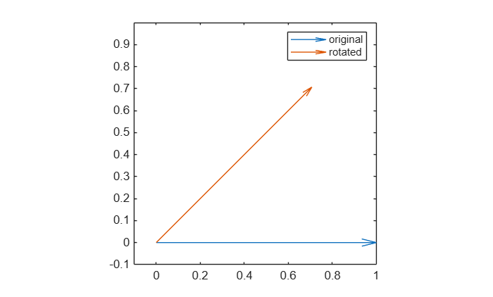
Use the quiver or quiver3 functions to visualize these rotations.
myThetaDegrees = 45; % degrees
myTheta = myThetaDegrees * pi / 180;
z1 = 1; % initial vector
z2 = z1 * exp(sqrt(-1) * myTheta); % Rotate original vector by myTheta
hold off
quiver(0,0,real(z1),imag(z1),AutoScale=false)
axis equal;axis([-0.1 1 -0.1 1])
hold on
quiver(0,0,real(z2),imag(z2),0)
legend("original","rotated")
Specify orientation of comm.RayTracingChannel
Several System objects in wireless communications toolboxes require antenna orientation information. For example:
The
TransmitArrayOrientationAxesandReceiveArrayOrientationAxesproperties in thecomm.RayTracingChannelSystem object™ specify 3-by-3 rotation matrices to define the pointing direction.The
AntennaAngleproperty in thetxsiteandrxsiteobjects specifies a 2-by-1 vector that defines the azimuth and elevation in degrees.The
txsiteandrxsiteobjects also include theangleobject function to compute azimuth and elevation between two sites.
The comm.RayTracingChannel object includes a syntax that accepts the txsite and rxsite objects as arguments and performs this coordinate-system conversion. This example includes a local function, rotAzEl(azAngle,elAngle), to demonstrate how the ray tracing channel object performs the coordinate system conversion.
Output the coordinate system conversion from txsite to antenna array coordinates by using the comm.RayTracingChannel object syntax. Then use the rotAzEl local function to compute the rotation matrices, rotMat, for the TransmitArrayOrientationAxes property required by the ray tracing channel object. The two approaches achieve the same result.
myChan = comm.RayTracingChannel(comm.Ray,txsite(AntennaAngle=[azAngle;elAngle]),rxsite);
myChan.TransmitArrayOrientationAxes
ans = 3×3

    0.8529    -0.5000    -0.1504
    0.4924     0.8660    -0.0868
    0.1736          0     0.9848
rotMat = rotAzEl(azAngle,elAngle)
rotMat = 3×3

    0.8529    -0.5000    -0.1504
    0.4924     0.8660    -0.0868
    0.1736          0     0.9848
Physically Steering Antennas
Antennas placed in a setting must define an initial position and orientation with respect that location and scene. This example shows an antenna array whose element phases are adjusted to form an electronically steered beam. Alternately the antenna may be mounted in a fixed unchanging orientation or a gimbal that allows it to be physically steered. This code sample uses Cartesian coordinates with ENU coordinate system convention, but the concepts apply when working with geographic coordinates. When starting with geographic coordinates, functions such as geodetic2enu (Mapping Toolbox), ecefOffset (Mapping Toolbox), and latlon2local (Automated Driving Toolbox) may be used to convert to Cartesian and then continue as above.
Define the transmitter and receiver location as TxLoc and RxLoc, respectively. Represent the separation between the transmitter and receiver by the vector v. The transmit and receive antenna locations are defined but orientation with respect to one another is not defined.
TxLoc = [10 2 0];
RxLoc = [1 -1 -5];
v = RxLoc - TxLoc
v = 1×3

    -9    -3    -5
Given the transmitter and receiver positions, compute the azimuth and elevation angles such that the antennas point directly at each other along the LOS path. Convert the displacement vector v to azimuth and elevation angles.
The azimuth angle is the angle from the x-axis to the projection of v onto the xy-plane.
TxAz = atan2(v(2),v(1))
TxAz =
-2.8198
The elevation angle is the angle between v and the xy-plane.
TxEl = atan2(v(3),sqrt(v(2)*v(2) + v(1)*v(1)))
TxEl =
-0.4850
Alternatively, you can use the cart2sph function to output the desired azimuth and elevation angles in radians.
[TxAz, TxEl]= cart2sph(v(1), v(2), v(3))
TxAz =
-2.8198
TxEl =
-0.4850
To point the transmitter and receiver antenna pattern peaks toward each other, the receiver must point in the opposite direction of the transmitter. Specifically, if the transmitter is oriented in the direction v, the receiver must be oriented in the direction –v.
RxAz = TxAz + pi
RxAz =
0.3218
RxEl = -TxEl
RxEl =
0.4850
Use siteviewer, together with the pattern and show functions to visualize transmitter and receiver antenna orientations and radiation patterns. Visualize a configuration with transmit and receive antennas not aligned. Adjust the antenna orientations to point toward each other, and then visualize the orientations again.
sv = siteviewer(SceneModel="none");
nelem = 50;
fc = 6e9;
lambda = physconst("LightSpeed") / fc;
txArray = phased.URA(Element=phased.ShortDipoleAntennaElement, ...
    Size=[nelem nelem], ...
    ElementSpacing=0.5*lambda);
myTx = txsite(TransmitterFrequency=fc, ...
    Antenna=txArray, ...
    CoordinateSystem="cartesian", ...
    AntennaPosition=TxLoc);
show(myTx,ShowAntennaHeight=false)
pattern(myTx)
rxArray = phased.URA(Element=phased.ShortDipoleAntennaElement, ...
    Size=[nelem nelem], ...
    ElementSpacing=0.5*lambda);
myRx = rxsite(Antenna=rxArray, CoordinateSystem="cartesian", ...
    AntennaPosition=RxLoc);
show(myRx,ShowAntennaHeight=false)
pattern(myRx,fc)
disp("Antennas not aligned")
Antennas not aligned
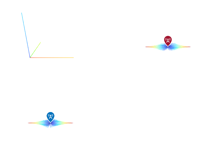
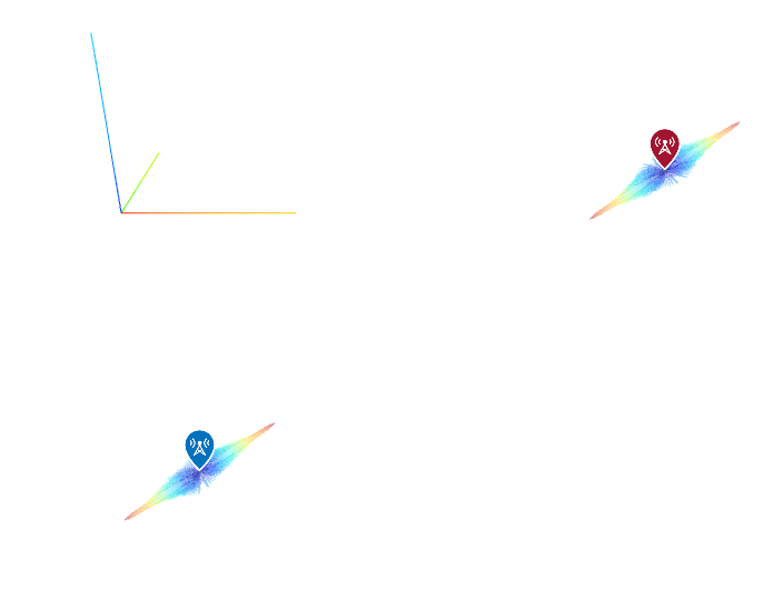
Use the AntennaAngle property of txsite and rxsite to point the antennas at each other.
myTx.AntennaAngle=[TxAz;TxEl]*180/pi; % Convert angles to degrees
myRx.AntennaAngle=[RxAz;RxEl]*180/pi; % Convert angles to degrees
pattern(myTx)
pattern(myRx,fc)
disp("Antennas now pointing at each other.")
Antennas now pointing at each other.
Electronic Beamsteering
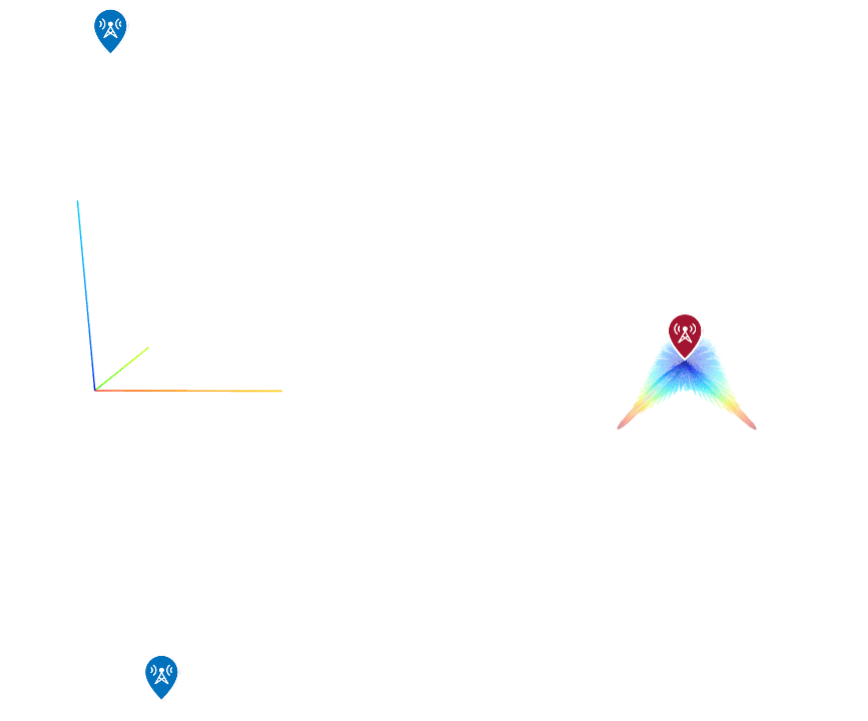
Suppose that the transmitter must retarget its beam dynamically during operation to point toward a second receiver. Define a second receiver location and electronically steer the transmit array between the two receivers. Use phased.SteeringVector (Phased Array System Toolbox) System object™ to create complex weights to use for electronically steering the transmitter array towards either receiver. The phased.SteeringVector object requires azimuth and elevation angles, so convert the transmitter-to-receiver displacement vectors into angular coordinates.
% Reset the scenario:
myTx.AntennaAngle = [0;0];
myRx.AntennaAngle = [0;0];
% Make new siteviewer
sv2 = siteviewer(SceneModel="none");
% Specify a second receiver
RxLoc2 = [1 -1  5];
myRx2 = rxsite(Antenna=rxArray, ...
    CoordinateSystem="cartesian", ...
    AntennaPosition=RxLoc2);
show(myRx2, ShowAntennaHeight=false)
show(myRx, ShowAntennaHeight=false)
show(myTx, ShowAntennaHeight=false)
svObj = phased.SteeringVector(SensorArray=txArray);
z = RxLoc2 - TxLoc;
az = atan2d(z(2),z(1))
az =
-161.5651
el = atan2d(z(3),sqrt(z(1)^2 + z(2)^2))
el =
27.7913
sv1 = svObj(fc,[az; -el]);
myTx.Antenna.Taper = conj(sv1); % conjugate because steering vector returns weights for receive beamforming
pattern(myTx)
disp("Tx array is electronically steered towards the 1st receiver (xyz = [1 -1 -5]).")
Tx array is electronically steered towards the 1st receiver (xyz = [1 -1 -5]).
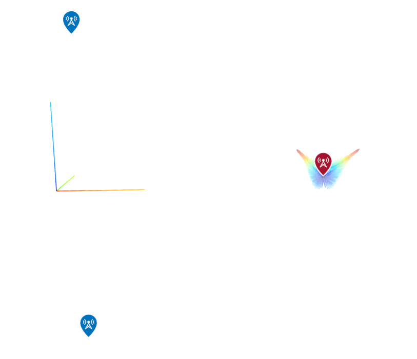
The extra lobe is due to an ambiguity in 2-D arrays. The delays are the same for a signal coming from the back side as from the front. Now steer towards the second receiver.
sv2 = svObj(fc,[az; el]);
myTx.Antenna.Taper = conj(sv2);
pattern(myTx)
disp("Tx array is electronically steered towards the second receiver (xyz = [1 -1  5]).")
Tx array is electronically steered towards the second receiver (xyz = [1 -1 5]).
Compute the rotation matrices for transmitter and receiver.
txrotmat = rotAzEl(az,el); % If Tx points north, then Rx must point south
rxrotmat = rotAzEl(az+180,-el); % if Tx points up, then Rx must point down
Antenna Polarization
For simulations that account for antenna polarization, you must consider antenna rotation. Define transmit and receive sites with identical rectangular panel arrays. For the propagation model consider LOS only.
txArray = phased.NRRectangularPanelArray( ...
    ElementSet={phased.NRAntennaElement(PolarizationAngle=45)});
txs = txsite(Antenna=txArray, ...
    CoordinateSystem="Cartesian", ...
    AntennaPosition=[0;0;0]);
rxArray = phased.NRRectangularPanelArray( ...
    ElementSet={phased.NRAntennaElement(PolarizationAngle=45)});
rxs = rxsite(Antenna=rxArray, ...
    CoordinateSystem="Cartesian", ...
    AntennaPosition=[1e3;0;0]);
pm = propagationModel("raytracing", ...
    MaxNumReflections=0, ...
    CoordinateSystem="cartesian");
losRay = raytrace(txs,rxs,pm);
Results below show this is a mistake because the transmit and receive polarization orientations must be configured to maintain polarization matching. The polarization mismatch for this configuration results in excessive path loss.
losRay{1}.PathLossans = 752.5642
Correct the mismatch by setting the receiver polarization to –45 degrees. The path loss is now representative of the distance between the transmitter and receiver.
rxArray = phased.NRRectangularPanelArray( ...
    ElementSet={phased.NRAntennaElement(PolarizationAngle=-45)});
rxs = rxsite(Antenna=rxArray, ...
    CoordinateSystem="Cartesian", ...
    AntennaPosition = [1e3;0;0]);
pm = propagationModel("raytracing", ...
    MaxNumReflections=0, ...
    CoordinateSystem="cartesian")
pm =
  RayTracing with properties:

       CoordinateSystem: "cartesian"
                 Method: "sbr"
      AngularSeparation: "medium"
      MaxNumReflections: 0
     MaxNumDiffractions: 0
    MaxAbsolutePathLoss: Inf
    MaxRelativePathLoss: 40
                 UseGPU: "off"
        SurfaceMaterial: "auto"
losRay = raytrace(txs,rxs,pm);
losRay{1}.PathLoss
ans = 98.0229
Polarization angle is defined with respect to the propagation direction. Because the transmitter and receiver face one another, equivalent physical polarization often requires opposite polarization-angle settings. Consequently, when a transmitter uses a polarization angle of +, the receiver typically requires a polarization angle of − to achieve polarization alignment.
txArray = phased.NRAntennaElement(PolarizationAngle = 45);
rxArray = phased.NRAntennaElement(PolarizationAngle = -45);
Similar notions apply if you are using more realistic antenna elements like phased.ShortDipoleAntennaElement (Phased Array System Toolbox) or phased.CrossedDipoleAntennaElement (Phased Array System Toolbox).
Summary
This example demonstrated how antenna orientation affects wireless link performance. It examines physical alignment, electronic beam steering, coordinate-system conversions, rotation matrices, and polarization alignment. Correctly accounting for each of these factors helps maximize received signal strength and maintain reliable link operation.
References
[1] Horizontal coordinate system - Wikipedia
[2] Aircraft principal axes - Wikipedia
Utility functions
function rotMat = rotAzEl(azAngle,elAngle) % Input angles in degrees
caz = cosd(azAngle);
saz = sind(azAngle);
cel = cosd(elAngle);
sel = sind(elAngle);
rotaz = [caz -saz 0; saz caz 0; 0 0 1]; % Azimuth or "yaw"
rotel = [cel 0 -sel; 0 1 0; sel 0 cel]; % Elevation or "pitch"
rotMat = rotaz * rotel;
end
Copyright 2026 The MathWorks, Inc.

