los
Display or compute line-of-sight (LOS) visibility status
Description
los(
specifies one or more name-value arguments. For example, the
site1,site2,Name=Value)ObstructedColor argument specifies the color that indicates
blocked visibility.
vis = los(site1,site2,Name,Value)
Examples
Create a transmitter site with an antenna of height 30 m and a receiver site at ground level.
tx = txsite("Name","MathWorks Apple Hill",...
      	"Latitude",42.3001,"Longitude",-71.3504,"AntennaHeight",30);
rx = rxsite("Name","MathWorks Lakeside", ...
   	    "Latitude",42.3021,"Longitude",-71.3764);
Plot the LOS between the two sites.
los(tx,rx)

Create a transmitter site with an antenna of height 30 m and two receiver sites with antennas at ground level.
tx = txsite("Name","MathWorks Apple Hill",...
      	"Latitude",42.3001,"Longitude",-71.3504,"AntennaHeight",30);

names = ["Fenway Park","Bunker Hill Monument"];
lats = [42.3467,42.3763];
lons = [-71.0972,-71.0611];
Create the receiver site array.
rxs = rxsite("Name", names,...
      "Latitude",lats,...
      "Longitude",lons);
Plot the LOSs to the receiver sites. The red portion of the LOS represents obstructed visibility.
los(tx,rxs)

Import and view an STL file. The file models a small conference room with one table and four chairs.
viewer = siteviewer("SceneModel","conferenceroom.stl");
Create a transmitter site near the upper corner of the room and a receiver site above the table. Specify the position using Cartesian coordinates in meters.
tx = txsite("cartesian", ...
    "AntennaPosition",[-1.46; -1.42; 2.1]);
rx = rxsite("cartesian", ...
    "AntennaPosition",[0.3; 0.3; 0.85]);
Plot the LOS between the transmitter and the receiver.
los(rx,tx)
Pan by left-clicking, zoom by right-clicking or by using the scroll wheel, and rotate the visualization by clicking the middle button and dragging or by pressing Ctrl and left-clicking and dragging.

Perform ray tracing in Chicago and return the rays in comm.Ray objects. Then, display the rays without performing the ray tracing analysis again.
Launch Site Viewer with buildings in Chicago. For more information about the OpenStreetMap® file, see [1].
viewer = siteviewer(Buildings="chicago.osm");
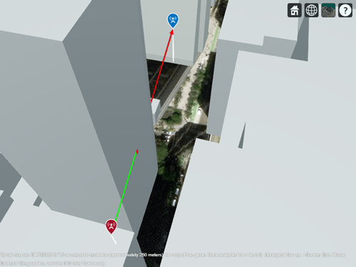
Create a transmitter site on one building and a receiver site on another building. Show the line-of-sight path between the sites using the los function.
tx = txsite(Latitude=41.8800, ...
    Longitude=-87.6295, ...
    TransmitterFrequency=2.5e9);
rx = rxsite(Latitude=41.881352, ...
    Longitude=-87.629771, ...
    AntennaHeight=30);
los(tx,rx)

Create a ray tracing propagation model, which MATLAB® represents using a RayTracing object. By default, the model uses the SBR method and calculates propagation paths with up to two reflections.
pm = propagationModel("raytracing");Perform the ray tracing analysis. The raytrace function returns a cell array containing the comm.Ray objects.
rays = raytrace(tx,rx,pm)
rays = 1×1 cell array
    {1×3 comm.Ray}
View the properties of the first ray object.
rays{1}(1)ans =
Ray with properties:
PathSpecification: 'Locations'
CoordinateSystem: 'Geographic'
TransmitterLocation: [3×1 double]
ReceiverLocation: [3×1 double]
LineOfSight: 0
Interactions: [1×1 struct]
Frequency: 2.5000e+09
PathLossSource: 'Custom'
PathLoss: 92.7686
PhaseShift: 1.2945
Read-only properties:
PropagationDelay: 5.7088e-07
PropagationDistance: 171.1462
AngleOfDeparture: [2×1 double]
AngleOfArrival: [2×1 double]
NumInteractions: 1
Close Site Viewer.
close(viewer)
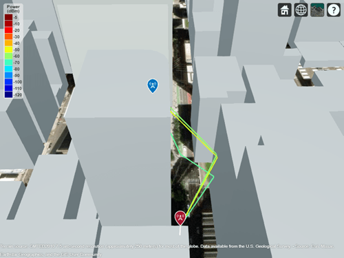
Create another Site Viewer with the same buildings, transmitter site, and receiver site. Then, display the propagation paths. Alternatively, you can plot individual paths by specifying a single ray object, for example rays{1}(2).
siteviewer(Buildings="chicago.osm");
show(tx)
show(rx)
plot(rays{1},Type="power", ...
    TransmitterSite=tx,ReceiverSite=rx)

Appendix
[1] The OpenStreetMap file is downloaded from https://www.openstreetmap.org, which provides access to crowd-sourced map data all over the world. The data is licensed under the Open Data Commons Open Database License (ODbL), https://opendatacommons.org/licenses/odbl/.
Input Arguments
Name-Value Arguments
Specify optional pairs of arguments as
Name1=Value1,...,NameN=ValueN, where Name is
the argument name and Value is the corresponding value.
Name-value arguments must appear after other arguments, but the order of the
pairs does not matter.
Before R2021a, use commas to separate each name and value, and enclose
Name in quotes.
Example: 'ObstructedColor','blue'
Plot color for successful visibility, specified as one of the following:
An RGB triplet whose elements specify the intensities of the red, green, and blue components of the color. The intensities must be in the range
[0,1]; for example,[0.4 0.6 0.7].A character vector such as
'red'or'r'.A string scalar such as
"red"or"r".
This table contains the color names and equivalent RGB triplets for some common colors.
| Color Name | Short Name | RGB Triplet | Appearance |
|---|---|---|---|
"red" | "r" | [1 0 0] |
|
"green" | "g" | [0 1 0] |
|
"blue" | "b" | [0 0 1] |
|
"cyan"
| "c" | [0 1 1] |
|
"magenta" | "m" | [1 0 1] |
|
"yellow" | "y" | [1 1 0] |
|
"black" | "k" | [0 0 0] |
|
"white" | "w" | [1 1 1] |
|
Plot color for blocked visibility, specified as one of the following:
An RGB triplet whose elements specify the intensities of the red, green, and blue components of the color. The intensities must be in the range
[0,1]; for example,[0.4 0.6 0.7].A character vector such as
'red'or'r'.A string scalar such as
"red"or"r".
This table contains the color names and equivalent RGB triplets for some common colors.
| Color Name | Short Name | RGB Triplet | Appearance |
|---|---|---|---|
"red" | "r" | [1 0 0] |
|
"green" | "g" | [0 1 0] |
|
"blue" | "b" | [0 0 1] |
|
"cyan"
| "c" | [0 1 1] |
|
"magenta" | "m" | [1 0 1] |
|
"yellow" | "y" | [1 1 0] |
|
"black" | "k" | [0 0 0] |
|
"white" | "w" | [1 1 1] |
|
Resolution of sample locations used to compute line-of-sight
visibility, specified as "auto" or a numeric scalar
expressed in meters. Resolution defines the distance
between samples on the great circle path using a spherical Earth model.
If Resolution is "auto", the
function computes a value based on the distance between the
sites.
Map for visualization or surface data, specified as a siteviewer
object, a triangulation object, a string scalar, or a character vector.
Valid and default values depend on the coordinate system.
| Coordinate System | Valid Map Values | Default Map Value |
|---|---|---|
"geographic" |
|
|
"cartesian" |
|
|
a Alignment of boundaries and region labels are a presentation of the feature provided by the data vendors and do not imply endorsement by MathWorks®. | ||
In most cases, if you specify this argument as a value other than a siteviewer or
"none", then you must also specify an output argument.
Output Arguments
Status of LOS visibility, returned as logical 1
(true) or 0
(false). If there are multiple target sites, the
function returns a logical array of size
n-by-1.
Limitations
The accuracy of the LOS visibility status can be limited at large distances due to floating-point precision.
Version History
Introduced in R2019b
MATLAB Command
You clicked a link that corresponds to this MATLAB command:
Run the command by entering it in the MATLAB Command Window. Web browsers do not support MATLAB commands.
Select a Web Site
Choose a web site to get translated content where available and see local events and offers. Based on your location, we recommend that you select: .
You can also select a web site from the following list
How to Get Best Site Performance
Select the China site (in Chinese or English) for best site performance. Other MathWorks country sites are not optimized for visits from your location.
Americas
- América Latina (Español)
- Canada (English)
- United States (English)
Europe
- Belgium (English)
- Denmark (English)
- Deutschland (Deutsch)
- España (Español)
- Finland (English)
- France (Français)
- Ireland (English)
- Italia (Italiano)
- Luxembourg (English)
- Netherlands (English)
- Norway (English)
- Österreich (Deutsch)
- Portugal (English)
- Sweden (English)
- Switzerland
- United Kingdom (English)