coverage
Display or compute coverage map
Syntax
Description
coverage( displays the coverage map
for the specified transmitter site in the current Site Viewer. Each colored contour
of the map defines an area where the corresponding signal strength is transmitted to
the mobile receiver.txs)
The CoordinateSystem property of the transmitter site must be
"geographic".
coverage(
displays the coverage map using information from the specified receiver site. The
function uses the receiver site to calculate the receiver gain and the receiver
antenna height, but does not use the latitude or longitude of the receiver site. For
more information about the receiver gain and the receiver antenna height, see the
txs,rx)ReceiverGain and ReceiverAntennaHeight
name-value arguments.
coverage(___,
displays the coverage map using additional options specified by name-value
arguments.Name=Value)
Examples
Create a transmitter site at MathWorks headquarters.
tx = txsite(Name="MathWorks",Latitude=42.3001,Longitude=-71.3503);Show the coverage map.
coverage(tx)

Create a transmitter site at MathWorks headquarters.
tx = txsite(Name="MathWorks",Latitude=42.3001,Longitude=-71.3503);Create a receiver site at Fenway Park with an antenna height of 1.2 m and system loss of 10 dB.
rx = rxsite(Name="Fenway Park",Latitude=42.3467,Longitude=-71.0972, ...
    AntennaHeight=1.2,SystemLoss=10);
Calculate the coverage area of the transmitter using a close-in propagation model.
coverage(tx,rx,PropagationModel="closein")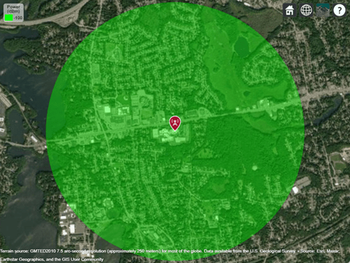
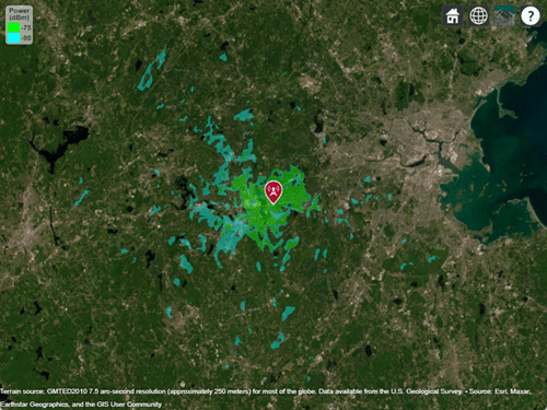
Define strong and weak signal strengths with corresponding colors.
strongSignal = -75;
strongSignalColor = "green";
weakSignal = -90;
weakSignalColor = "cyan";
Create a transmitter site and display the coverage map.
tx = txsite(Name="MathWorks", ...
    Latitude=42.3001, ...
    Longitude=-71.3503);
coverage(tx,SignalStrengths=[strongSignal,weakSignal], ...
    Colors=[strongSignalColor,weakSignalColor])
Define the names and the locations of sites around Boston.
names = ["Fenway Park","Faneuil Hall","Bunker Hill Monument"];
lats = [42.3467,42.3598,42.3763];
lons = [-71.0972,-71.0545,-71.0611];
Create the transmitter site array.
txs = txsite(Name=names, ...
    Latitude=lats, ...
    Longitude=lons, ...
    TransmitterFrequency=2.5e9);
Display the combined coverage map for multiple signal strengths, using close-in propagation model.
coverage(txs,"close-in",SignalStrengths=-100:5:-60)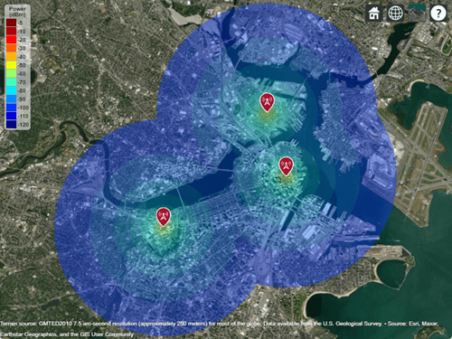
Launch Site Viewer using buildings in Chicago. For more information about the OpenStreetMap® file, see [1].
viewer = siteviewer(Buildings="chicago.osm");Create a transmitter site on a building.
tx = txsite(Latitude=41.8800, ...
    Longitude=-87.6295, ...
    TransmitterFrequency=2.5e9);
show(tx)
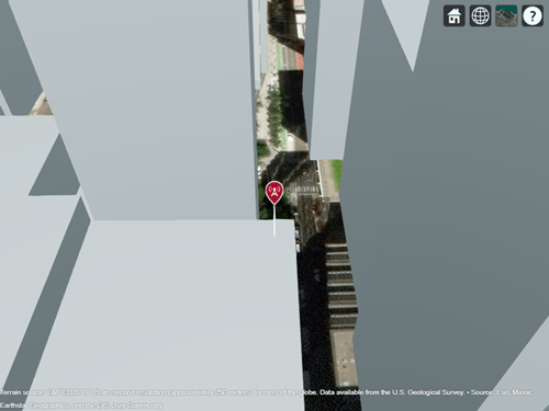
Coverage Map Using Longley-Rice Propagation Model
Create a coverage map of the city using the Longley-Rice propagation model.
coverage(tx,SignalStrengths=-100:-5,MaxRange=250,Resolution=1)
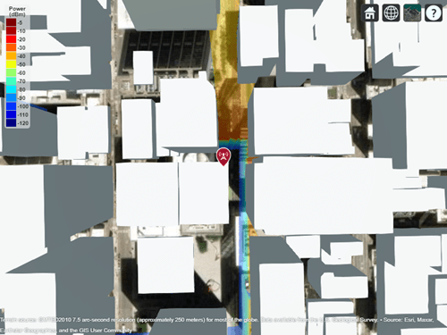
Longley-Rice models over-the-rooftops propagation along vertical slices and obstructions tend to dominate the coverage region.
Coverage Map Using Ray Tracing Propagation Model and Image Method
Create a ray tracing propagation model, which MATLAB® represents using a RayTracing object. Configure the model to use the image method and to find propagation paths with up to 1 surface reflection.
pmImage = propagationModel("raytracing",Method="image", ...
    MaxNumReflections=1);
Create a coverage map of the city using the transmitter site and the ray tracing propagation model.
coverage(tx,pmImage,SignalStrengths=-100:-5, ...
    MaxRange=250,Resolution=2)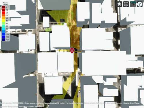
This coverage map shows new regions that are in service due to reflected propagation paths.
Coverage Map Using Ray Tracing Propagation Model and SBR Method
Create another ray tracing propagation model. This time, configure the model to use the shooting and bouncing rays (SBR) method and to find propagation paths with up to 2 surface reflections. The SBR method is generally faster than the image method.
pmSBR = propagationModel("raytracing",Method="sbr", ...
    MaxNumReflections=2);
Create an updated coverage map of the city.
coverage(tx,pmSBR,SignalStrengths=-100:-5, ...
    MaxRange=250,Resolution=2)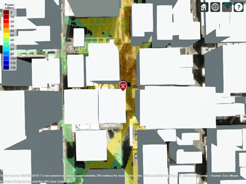
This coverage map shows new regions that are in service due to the additional reflected propagation paths.
Appendix
[1] The OpenStreetMap file is downloaded from https://www.openstreetmap.org, which provides access to crowd-sourced map data all over the world. The data is licensed under the Open Data Commons Open Database License (ODbL), https://opendatacommons.org/licenses/odbl/.
Input Arguments
Name-Value Arguments
Specify optional pairs of arguments as
Name1=Value1,...,NameN=ValueN, where Name is
the argument name and Value is the corresponding value.
Name-value arguments must appear after other arguments, but the order of the
pairs does not matter.
Example: coverage(txs,Type="efield") specifies the signal
strength units as electric field strength units (dBμV/m).
Before R2021a, use commas to separate each name and value, and enclose
Name in quotes.
Example: coverage(txs,"Type","efield") specifies the signal
strength units as electric field strength units (dBμV/m).
General
For Plotting Coverage
Maximum range of the coverage map from each transmitter site,
specified as a positive numeric scalar in m representing great circle
distance. MaxRange defines the region of interest
on the map to plot. The default value is automatically computed based on
the type of propagation model.
| Type of Propagation Model | Default Maximum Range |
|---|---|
| Atmospheric or empirical | Range of minimum value in
SignalStrengths |
| Terrain | The minimum of 30 km and the distance to the furthest building |
| Ray tracing | 500 m |
For more information about the types of propagation models, see Choose a Propagation Model.
Data Types: double
Resolution of the coverage map, specified as "auto"
or a numeric scalar in m. If the resolution is
"auto", the function computes the maximum value
scaled to MaxRange. Decreasing the resolution
increases the quality of the coverage map and the time required to
create it.
Data Types: char | string | double
Colors of filled contours on the coverage map, specified as one of these options:
An M-by-3 array of RGB triplets whose elements specify the intensities of the red, green, and blue components of the color. The intensities must be in the range
[0,1]; for example,[0.4 0.6 0.7].An array of strings such as
["red" "green" "blue"]or["r" "g" "b"].A cell array of character vectors such as
{'red','green','blue'}or{'r','g','b'}.
Colors are assigned element-wise to
SignalStrengths values for coloring the
corresponding filled contours.
Colors cannot be used with
ColorLimits or
Colormap.
This table contains the color names and equivalent RGB triplets for some common colors.
| Color Name | Short Name | RGB Triplet | Appearance |
|---|---|---|---|
"red" | "r" | [1 0 0] |
|
"green" | "g" | [0 1 0] |
|
"blue" | "b" | [0 0 1] |
|
"cyan"
| "c" | [0 1 1] |
|
"magenta" | "m" | [1 0 1] |
|
"yellow" | "y" | [1 1 0] |
|
"black" | "k" | [0 0 0] |
|
"white" | "w" | [1 1 1] |
|
Data Types: char | string | double
Color limits for colormap, specified as a two-element vector of the
form [cmin cmax]. The value of
cmin must be less than cmax.
The color limits indicate the signal level values that map to the first and last colors on the colormap.
The default value is [-120 -5] if the
Type is "power" and
[20 135] if Type is
"efield".
ColorLimits cannot be used with
Colors.
Data Types: double
Colormap for the filled contours, specified as a colormap name or as an M-by-3 array of RGB triplets that define M individual colors.
This table lists the colormap names.
| Colormap Name | Color Scale |
|---|---|
|
|
|
|
|
|
|
|
|
|
|
|
|
|
|
|
|
|
|
|
|
|
|
|
|
|
|
|
|
|
|
|
|
|
|
|
|
|
|
|
|
|
|
|
Colormap cannot be used with
Colors.
Data Types: char | string | double
Show signal strength color legend on map, specified as
true or false.
Data Types: logical
Transparency of coverage map, specified as a numeric scalar in the
range 0 to 1. 0
is transparent and 1 is opaque.
Data Types: double
Output Arguments
Limitations
When you specify a RayTracing object as
input to the coverage function, the value of the
MaxNumDiffractions property must be 0 or
1.
References
[1] International Telecommunications Union Radiocommunication Sector. Effects of Building Materials and Structures on Radiowave Propagation Above About 100MHz. Recommendation P.2040. ITU-R, approved August 23, 2023. https://www.itu.int/rec/R-REC-P.2040/en.
[2] International Telecommunications Union Radiocommunication Sector. Electrical Characteristics of the Surface of the Earth. Recommendation P.527. ITU-R, approved September 27, 2021. https://www.itu.int/rec/R-REC-P.527/en.
[3] Mohr, Peter J., Eite Tiesinga, David B. Newell, and Barry N. Taylor. “Codata Internationally Recommended 2022 Values of the Fundamental Physical Constants.” NIST, May 8, 2024. https://www.nist.gov/publications/codata-internationally-recommended-2022-values-fundamental-physical-constants.
[4] "IEEE Standard Definitions of Terms for Antennas." IEEE Std 145-2013 (Revision of IEEE Std 145-1993), March 2014, 1–50. https://doi.org/10.1109/IEEESTD.2014.6758443.
Extended Capabilities
Version History
Introduced in R2019b1 Alignment of boundaries and region labels are a presentation of the feature provided by the data vendors and do not imply endorsement by MathWorks®.