Bit Error Rate Analysis
Analyze BER performance of communications systems
Description
The Bit Error Rate Analysis app calculates the bit error rate (BER) as a function of the energy per bit to noise power spectral density ratio (Eb/N0). Using this app, you can:
Generate BER data for a communications system and analyze performance using:
Monte Carlo simulations of MATLAB® functions and Simulink® models.
Theoretical closed-form expressions for selected types of communications systems.
Run systems contained in MATLAB simulation functions or Simulink models. After you create a function or model that simulates the system, the Bit Error Rate Analysis app iterates over your choice of Eb/N0 values and collects the results.
Plot one or more BER data sets on a single set of axes. You can graphically compare simulation data with theoretical results or simulation data from a series of communications system models.
Fit a curve to a set of simulation data.
Plot confidence levels of simulation data.
Send BER data to the MATLAB workspace or to a file for further processing.
For more information, see Analyze Performance with Bit Error Rate Analysis App.
Open the Bit Error Rate Analysis App
MATLAB Toolstrip: On the Apps tab, under Wireless Communications, click the app icon.
MATLAB command prompt: Enter
bertool.
Examples
Generate a theoretical estimate of BER performance for a 16-QAM link in AWGN.
Open the Bit Error Rate Analysis app.
bertool
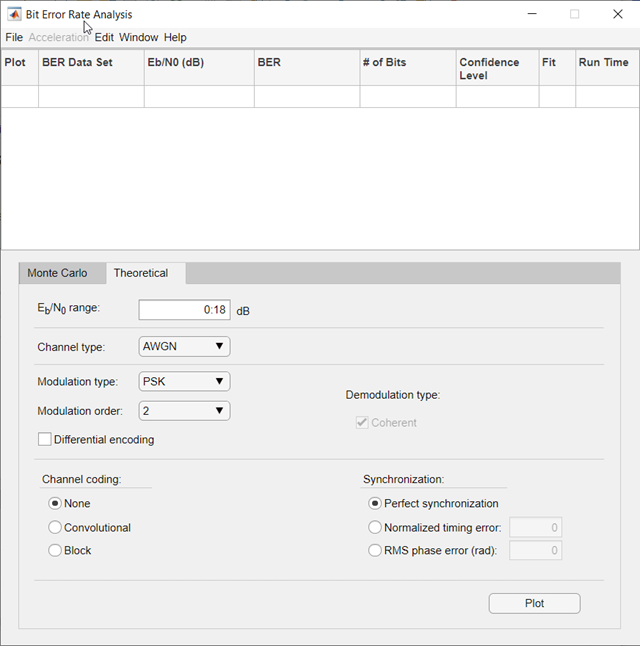
On the Theoretical tab, set these parameters to the specified values:
Eb/N0
range to 0:10, Modulation
type to QAM, and Modulation
order to 16.
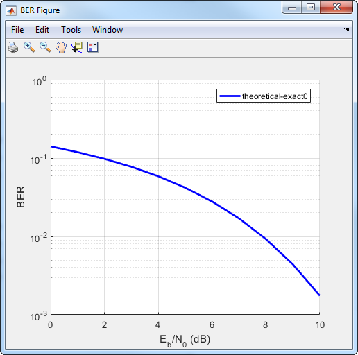
Plot the BER curve by clicking Plot.
Simulate the BER by using a custom MATLAB function. By default, the app uses the
viterbisim.m simulation.
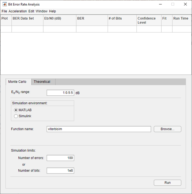
Open the Bit Error Rate Analysis app.
bertool
On the Monte Carlo tab, set the Eb/N0
range parameter to 1:.5:6. Run the
simulation and plot the estimated BER values by clicking
Run.
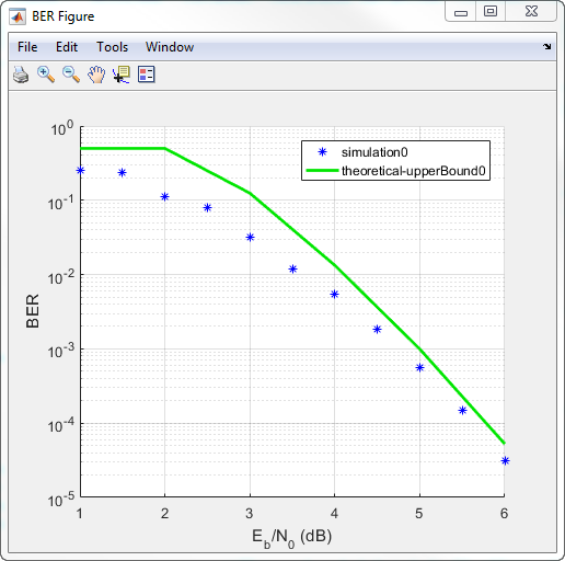
On the Theoretical tab, set Eb/N0
range to 1:6 and set Modulation
order to 4. Enable convolutional
coding by selecting Convolutional. Click
Plot to add the theoretical upper bound of the BER
curve to the plot.
Add code to the simulation function template given in the Template for Simulation Function topic to run in the Monte Carlo tab of the Bit Error Rate Analysis.
Prepare Function
Copy the template from the Template for Simulation Function topic into a new MATLAB file in the MATLAB Editor. Save the file in a folder on your MATLAB path, using the file name
bertool_simfcn.
Place lines of code that initialize parameters or create objects used in
the simulation in the template section marked Set up initial
parameters. This code maps simulation variables to the
template input arguments. For example, snr maps to
EbNo.
% Set up initial parameters.
siglen = 1000; % Number of bits in each trial
M = 2;         % DBPSK is binary
snr = EbNo;    % Because of binary modulation

% Create an ErrorRate calculator System object to compare
% decoded symbols to the original transmitted symbols.
errorCalc = comm.ErrorRate;
Place the code for the core simulation tasks in the template section
marked Proceed with simulation. This code includes the
core simulation tasks, after all setup work has been performed.
    msg = randi([0,M-1],siglen,1); % Generate message sequence
    txsig = dpskmod(msg,M);        % Modulate
    hChan.SignalPower = ...        % Calculate and assign signal power
        (txsig'*txsig)/length(txsig);
    rxsig = awgn(txsig,snr,'measured'); % Add noise
    decodmsg = dpskdemod(rxsig,M);      % Demodulate
    berVec = errorCalc(msg,decodmsg);   % Calculate BER
    totErr = totErr + berVec(2);
    numBits = numBits + berVec(3);
After you insert these two code sections into the template, the
bertool_simfcn function is compatible with the
Bit Error Rate Analysis app. The resulting code resembles
this code segment.
function [ber,numBits] = bertool_simfcn(EbNo,maxNumErrs,maxNumBits,varargin)
%
%   See also BERTOOL and VITERBISIM.

% Copyright 2020 The MathWorks, Inc.

% Initialize variables related to exit criteria.
totErr = 0;  % Number of errors observed
numBits = 0; % Number of bits processed

% --- Set up the simulation parameters. ---
% --- INSERT YOUR CODE HERE.
% Set up initial parameters.
siglen = 1000; % Number of bits in each trial
M = 2;         % DBPSK is binary.
snr = EbNo;    % Because of binary modulation
% Create an ErrorRate calculator System object to compare
% decoded symbols to the original transmitted symbols.
errorCalc = comm.ErrorRate;

% Simulate until the number of errors exceeds maxNumErrs
% or the number of bits processed exceeds maxNumBits.
while((totErr < maxNumErrs) && (numBits < maxNumBits))

    % Check if the user clicked the Stop button of BERTool.
    if isBERToolSimulationStopped(varargin{:})
      break
    end

    % --- Proceed with the simulation.
    % --- Update totErr and numBits.
    % --- INSERT YOUR CODE HERE.
    msg = randi([0,M-1],siglen,1); % Generate message sequence
    txsig = dpskmod(msg,M);        % Modulate
    hChan.SignalPower = ...        % Calculate and assign signal power
        (txsig'*txsig)/length(txsig);
    rxsig = awgn(txsig,snr,'measured'); % Add noise
    decodmsg = dpskdemod(rxsig,M);      % Demodulate
    berVec = errorCalc(msg,decodmsg);   % Calculate BER
    totErr = totErr + berVec(2);
    numBits = numBits + berVec(3);
end % End of loop

% Compute the BER.
ber = totErr/numBits;
The function has inputs to specify the app and scalar quantities for
EbNo, maxNumErrs, and
maxNumBits that are provided by the app. The Bit
Error Rate Analysis app is an input because the function monitors
and responds to the stop command in the app. The
bertool_simfcn function excludes code related to
plotting, curve fitting, and confidence intervals because the Bit Error
Rate Analysis app enables you to do similar tasks interactively
without writing code.
Use Prepared Function
Run bertool_simfcn in the Bit Error Rate
Analysis app.
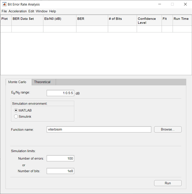
Open the Bit Error Rate Analysis app, and then select the Monte Carlo tab.
Set these parameters to the specified values:
Eb/N0
range to 0:10, Simulation
environment to MATLAB, Function
name to bertool_simfcn, Number
of errors to 5, and Number of
bits to 1e8.
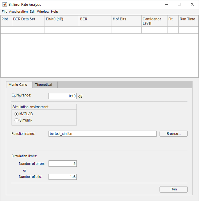
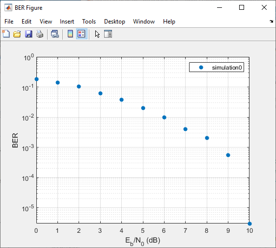
Click Run.
The Bit Error Rate Analysis app computes the results and then
plots them. In this case, the results do not appear to fall along a smooth
curve because the simulation required only five errors for each value in
EbNo.
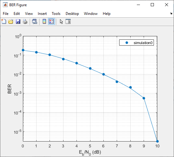
Fit a curve to the series of points in the BER Figure window, by selecting the Fit parameter in the data viewer.

The Bit Error Rate Analysis app plots the fitted curve, as shown in this figure.
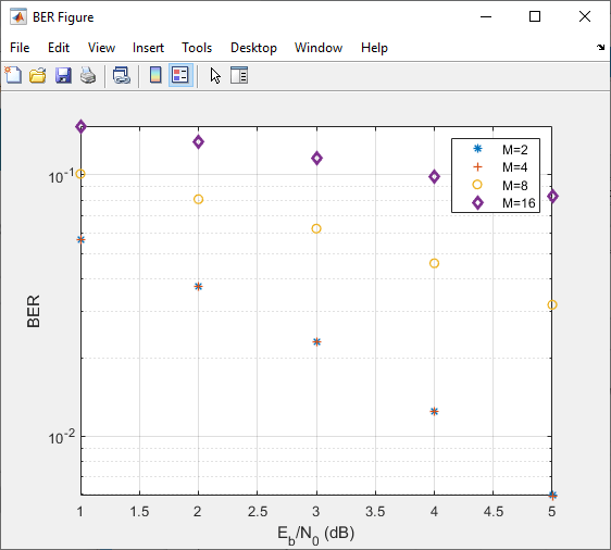
Use the Bit Error Rate Analysis app to compute the BER as a function of . The app analyzes performance with either Monte Carlo simulations of MATLAB® functions and Simulink® models or theoretical closed-form expressions for selected types of communications systems. The code in the mpsksim.m function provides an M-PSK simulation that you can run from the Monte Carlo tab of the app.
Open the Bit Error Rate Analysis app from the Apps tab or by running the bertool function in the MATLAB command window.
On the Monte Carlo tab, set the range parameter to 1:1:5 and the Function name parameter to mpsksim.
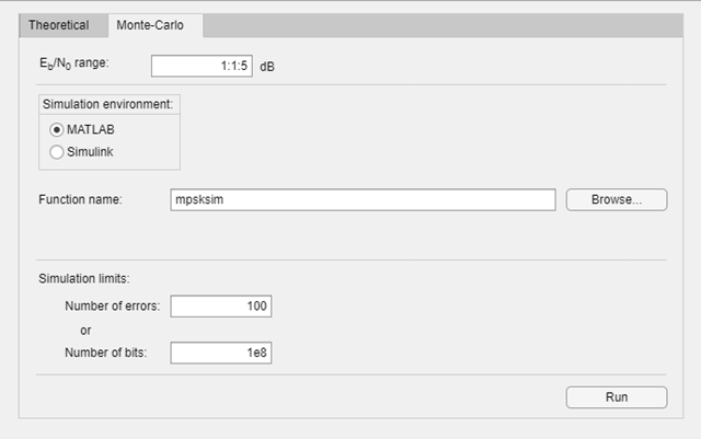
Open the mpsksim function for editing, set M=2, and save the changed file.
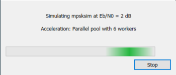
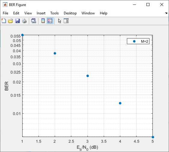
Run the mpsksim.m function as configured by clicking Run on the Monte Carlo tab in the app.
After the app simulates the set of points, update the name of the BER data set results by selecting simulation0 in the BER Data Set field and typing M=2 to rename the set of results. The legend on the BER figure updates the label to M=2.


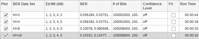
Update the value for M in the mpsksim function, repeating this process for M = 4, 8, and 16. For example, these figures of the Bit Error Rate Analysis app and BER Figure window show results for varying M values.
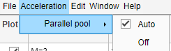
Parallel SNR Sweep Using Bit Error Rate Analysis App
The default configuration for the Monte Carlo processing of the Bit Error Rate Analysis app automatically uses parallel pool processing to process individual points when you have the Parallel Computing Toolbox™ software but for the processing of your simulation code:
Copyright 2020 The MathWorks, Inc.
This example shows you how to use a Simulink® model to run in the Monte Carlo tab of the Bit Error Rate Analysis app and compare the BER performance of the Simulink® simulation results with theoretical BER results.
Prepare Model and App
Open the example to load the doc_bpsk model into a working folder on your computer.

Open the doc_bpsk model from the working directory it was downloaded to and the Bit Error Rate Analysis app from the apps gallery. Parameters that control the range, load the model, save the results, and set the stopping criteria for each BER iteration must align in the Bit Error Rate Analysis app and in the Simulink® model.
On the Monte Carlo tab in the app,
The range parameter maps to the variable name
EbNo.The Number of errors parameter maps to the variable name
maxNumErrs.The Number of bits parameter maps to the variable name
maxNumBits.Select Simulink for the Simulation environment. For Model name enter
doc_bspkand for BER variable name enterBER.
In the model, the PreloadFcn callback function initializes variables for EbNo, maxNumErrs, and maxNumBits that set block parameters in the model. For more information on the PreloadFcn callback function, see Model Callbacks (Simulink). To ensure the app will control the model, in the model confirm that the:
AWGN Channel block has Es/No (dB) set to
EbNo. For BPSK modulation, is equivalent to .Error Rate Calculation block has Target number of errors set to
maxNumErrs, and Maximum number of symbols set tomaxNumBits.To Workspace block has Variable name set to
BER.In the model Simulation, set Stop Time to
Inf.
Use Prepared Model
In the Monte Carlo tab of the Bit Error Rate Analysis app, set:
range to
0:9Number of errors to
100Number of bits to
1e8
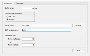
Click Run. The Bit Error Rate Analysis app computes the results and then plots them.
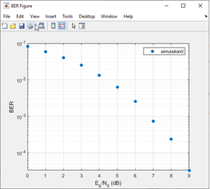
Compare these simulation results with the theoretical results, by clicking the Theoretical tab in the app and setting Eb/N0 range to 0:9.

Click Plot.
The app plots the theoretical curve in the BER Figure window along with the earlier simulation results.

Parameters
Tips
You can stop the simulation by clicking Stop on the Monte Carlo Simulation dialog box.