Main Content

berfit

Fit curve to nonsmooth empirical BER data

Description

fitber = berfit(empEbNo,empber) fits a curve to the empirical BER data, empber, and returns a vector of fitted BER points. The values in empber and fitber correspond to the empirical energy per bit to noise power spectral density ratio (Eb/N0) values given by empEbNo. For a general description of unconstrained nonlinear optimization, see [1].

Note

The berfit function is intended for curve fitting or interpolation (not extrapolation). Extrapolating BER data beyond an order of magnitude below the smallest empirical BER value is inherently unreliable.

example

fitber = berfit(empEbNo,empber,fitEbNo) specifies a vector of Eb/N0 values to use when fitting a curve to the empirical BER data in empber that correspond to the empirical Eb/N0 values in empEbNo.

fitber = berfit(empEbNo,empber,fitEbNo,options) specifies a structure to override the default options used for optimization.

fitber = berfit(empEbNo,empber,fitEbNo,options,fittype) specifies the closed-form function used to fit the empirical data. If you do not want to override the default options for optimization, specify options as [ ].

[fitber,fitprops] = berfit(___) returns the fitprops structure with fields that describe the properties of the curve fit. Use any input argument combination from previous syntaxes.

berfit(___) plots the empirical and fitted BER data.

berfit(empEbNo,empber,fitEbNo,options,'all') plots the empirical and fitted BER data from all possible settings of fittype that are valid. If you do not want to override the default options for optimization, specify options as [ ].

Note

To be valid a fit must conform to these criteria, otherwise it is rejected.

  • real-valued

  • monotonically decreasing

  • greater than or equal to 0 and less than or equal to 1

Examples

collapse all

This example shows the use of the berfit function using hard-coded or theoretical BER points for simplicity. For an example that uses empirical BER data from a simulation, see Use Curve Fitting on Error Rate Plot.

Best Fit for Set of Sample Data

Define a range of Eb/N0 values and BER points. Use this data as inputs for the berfit function.

EbN0 = 0:13;
berdata = [.2 .15 .13 .12 .08 .09 .08 .07 .06 .04 .03 .02 .01 .004];
berfit(EbN0,berdata); 

Figure contains an axes object. The axes object with title BER vs. Eb/No with Best Curve Fit, xlabel Eb/No (dB), ylabel BER contains 2 objects of type line. One or more of the lines displays its values using only markers These objects represent Empirical BER, Poly Ratio Fit.

Plot Best Fit

The curve connects the points created by evaluating the fit expression at the specified Eb/N0 values. To make the curve look smoother, provide an input vector of Eb/N0 values for curve fitting in ascending order. This vector provides more points for plotting the curve and does not change the fit expression.

fitEbNo = 0:0.2:13;
berfit(EbN0,berdata,fitEbNo)

Figure contains an axes object. The axes object with title BER vs. Eb/No with Best Curve Fit, xlabel Eb/No (dB), ylabel BER contains 2 objects of type line. One or more of the lines displays its values using only markers These objects represent Empirical BER, Poly Ratio Fit.

Fit for BER Curve with Error Floor

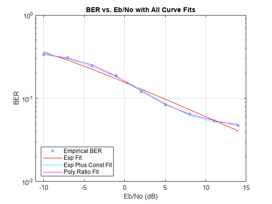
Run the berfit function using the 'all' option on empirical BER results for a simulation of BPSK data transmitted over a channel with a null (ch = [0.5 0.47]) and recovered by using a linear MMSE equalizer at the receiver for the Eb/N0 range [-10, 15]. Comparing the results of curve fitting methods

  • 'doubleExp+const' fit type does not provide a valid fit

  • 'exp' fit type does not work well for this data

  • 'exp+const' and 'polyRatio' fit types closely match the simulated data

EbN0 = -10:3:15;
empBER = [0.3361 0.3076 0.2470 0.1878 0.1212 0.0845 0.0650 0.0540 0.0474];
figure;
berfit(EbN0,empBER,[],[],'all');

Figure contains an axes object. The axes object with title BER vs. Eb/No with All Curve Fits, xlabel Eb/No (dB), ylabel BER contains 4 objects of type line. One or more of the lines displays its values using only markers These objects represent Empirical BER, Exp Fit, Exp Plus Const Fit, Poly Ratio Fit.

Use of options Input Structure and fitprops Output Structure

The 'notify' value for the display level causes the function to produce output when one of the attempted fits does not converge. The exitState field of the output structure indicates which fit type converges.

Generate theoretical BER results for 8-PSK data with a diversity order of 2 transmitted over a Rayleigh fading channel for the Eb/N0 range [3, 10] dB.

M = 8; EbN0 = 3:10;
berdata = berfading(EbN0,'psk',M,2); % Compute the theoretical BER
noisydata = berdata.*[.93 .92 1 .59 .08 .15 .01 .01];

Create the options structure by using the optimset function to configure display and notification of fit type results. Run exponential and polynomial ratio fit types.

options = optimset('display','notify');
disp('*** Trying exponential fit.') % Poor fit
*** Trying exponential fit.
[fitber1,fitprops1] = berfit(EbN0,noisydata,EbN0,...
   options,'exp')
 
Exiting: Maximum number of function evaluations has been exceeded
         - increase MaxFunEvals option.
         Current function value: 2.749919 
fitber1 = 1×8

    0.1247    0.0727    0.0376    0.0168    0.0064    0.0020    0.0005    0.0001

fitprops1 = struct with fields:
       fitType: 'exp'
        coeffs: [4x1 double]
      sumSqErr: 2.7499
     exitState: 'The maximum number of function evaluations has been exceeded'
     funcCount: 10001
    iterations: 6193

disp('*** Trying polynomial ratio fit.') % Good fit
*** Trying polynomial ratio fit.
[fitber2,fitprops2] = berfit(EbN0,noisydata,EbN0,...
   options,'polyRatio')
fitber2 = 1×8

    0.1701    0.0874    0.0407    0.0169    0.0060    0.0016    0.0003    0.0001

fitprops2 = struct with fields:
       fitType: 'polyRatio'
        coeffs: [6x1 double]
      sumSqErr: 2.3880
     exitState: 'The curve fit converged to a solution'
     funcCount: 554
    iterations: 331

Input Arguments

collapse all

Empirical Eb/N0 values in dB, specified as a vector with at least four elements. The element values in the vector must be in ascending order.

Data Types: single | double

Empirical BER data, specified as a vector with the same number of elements as input empEbNo. The values in empber correspond to the Eb/N0 values given by empEbNo.

Data Types: single | double

Eb/N0 values in dB for curve fitting, specified as a vector with element values in ascending order. The length of fitEbNo must equal or exceed that of input empEbNo.

Data Types: single | double

Override default options used for optimization, specified as a structure. The fields specified in the options structure are used by the fminsearch function. You can create the options structure by using the optimset function. This table describes the fields that are most relevant when using the berfit function. To use default options, you can specify this input as [ ].

FieldDescription
options.Display

Level of display.

  • 'off' (default) –- displays no output

  • 'iter' –- displays output at each iteration

  • 'final' –- displays only the final output

  • 'notify' –- displays output only if the function does not converge

options.MaxFunEvalsThe maximum number of function evaluations before optimization ceases. The default is 104.
options.MaxIterThe maximum number of iterations before optimization ceases. The default is 104.
options.TolFunThe termination tolerance for the closed-form function used to generate the fit. The default is 10-4.
options.TolXThe termination tolerance for the coefficient values of the closed-form function used to generate the fit. The default is 10-4.

Data Types: struct

Closed-form function used to fit the empirical data, specified as 'exp', 'exp+const', 'polyRatio', or 'doubleExp+const'. For more information, see Algorithms.

Data Types: char | string

Output Arguments

collapse all

Fitted BER points, returned as a vector. The BER is computed for each Eb/N0 setting specified by the input empEbNo vector.

Data Types: double

Fit properties, returned as a structure with these fields to describe the properties of the curve fit.

FieldDescription
fitprops.fitTypeThe closed-form function type used to generate the fit. Valid values include: 'exp', 'exp+const', 'polyRatio', or 'doubleExp+const'.
fitprops.coeffsThe coefficients used to generate the fit. If the function cannot find a valid fit, fitprops.coeffs is an empty vector.
fitprops.sumSqErrThe sum squared error between the log of the fitted BER points and the log of the empirical BER points.
fitprops.exitState

The exit condition of berfit. Valid values include:

  • 'The curve fit converged to a solution.'

  • 'The maximum number of function evaluations was exceeded.'

  • 'No desirable fit was found.'

fitprops.funcCountThe number of function evaluations used in minimizing the sum squared error function.
fitprops.iterationsThe number of iterations taken in minimizing the sum squared error function. This value is not necessarily equal to the number of function evaluations.

Data Types: struct

Algorithms

The berfit function fits the BER data using unconstrained nonlinear optimization via the fminsearch function. This table lists the closed-form functions that berfit considers based on the value of the fittype input argument. These functions were empirically found to provide close fits in a wide variety of situations, including exponentially decaying BERs, linearly varying BERs, and BER curves with error rate floors. In the functional expressions, x is a linear Eb/N0 value (not a dB value), and f(x) is the estimated BER.

fittype ValueFunctional Expression
'exp'

f(x)=a1exp[(xa2)a3a4]

'exp+const'

f(x)=a1exp[(xa2)a3a4]+a5

'polyRatio'

f(x)=a1x2+a2x+a3x3+a4x2+a5x+a6

'doubleExp+const'

a1exp[(xa2)a3a4]+a5exp[(xa6)a7a8]+a9

The sum squared error function that fminsearch attempts to minimize is

F=[log(empirical BER)log(fitted BER)]2

The fitted BER points are the values in the output fitber, and the sum is over the Eb/N0 points given in the input empEbNo. To avoid high-BER regions dominating the objective function, the sum squared equation uses the log of the BER values rather than the BER values themselves.

References

[1] Chapra, Steven C., and Raymond P. Canale. Numerical Methods for Engineers. Fourth Edition. New York, McGraw-Hill, 2002.

Version History

Introduced before R2006a

Go to top of page